Artificial Intelligence (AI) – Chih-Yu (Andrew) Lai's Website

Survival Rate Prediction Model for Startup Companies

Posted on 2020/05/16 | by andrewlai61616

This is an end semester project that I have done with my groupmates in college. In this study, we proposed a model to predict a startup company’s future condition using a deep multilayer perceptron (MLP) and decision tree. I mainly played the role for data quantification and literature review of this study. In our study, we built a prediction analysis model for startup companies. Furthermore, we identified what the key factors are and what influences will it have on the results. Our main hypothesis is that money, people and active days are the key factors. We built the prediction model from CrunchBase, which is the largest public database with relevant profiles about companies.

Data Quantification

For the data obtained, there are 4 groups of data that are quantified: country state, employee range, roles and countries. Regarding the states group (which only exists in USA and Canada), we think that different states have different impacts on the survival rate of a startup. A lookup table for scoring of states is defined [1][2][3]. The original data for employee quantities are a range between two numbers (e.g. 101-250). These are transformed into the average of the upper and lower bound. Employees of 10000+ are defined to be 15000. For the roles group, the data “company” is arbitrarily defined as 0.1 and “company, investor” is defined as 0.9. This is because we regard a company as wealthier and influential when it also plays a role of an investor, compared with only being a company. The other roles are transformed to 0.5. The impact of country on startup environment is also studied [4] and scores from 0.329 to 0.947 are given to countries that have above 300 startup companies in record.

Table 1. Company status and scores of 23 countries.

Country	Closed	Operating	Acquired	IP O	Score
BRA	4.7%	90.1%	4.5%	0.6%	0.329
ESP	5.3%	86.8%	7.3%	0.7%	0.333
FIN	3.6%	82.9%	12.6%	0.9%	0.340
ITA	2.9%	89.5%	6.6%	1.0%	0.345
RUS	6.0%	87.5%	4.7%	1.8%	0.379
KOR	4.9%	89.0%	3.5%	2.6%	0.411
BEL	4.3%	80.6%	12.3%	2.8%	0.419
NLD	3.6%	83.5%	10.1%	2.8%	0.421
GBR	5.2%	81.4%	10.5%	2.9%	0.423
DEU	5.5%	78.7%	12.9%	2.9%	0.423
IRL	5.8%	78.9%	12.0%	3.3%	0.443
DNK	4.4%	79.6%	12.1%	3.9%	0.466
CHE	2.7%	83.3%	10.0%	4.0%	0.471
SWE	3.9%	82.3%	9.8%	4.0%	0.473
USA	8.1%	69.3%	18.5%	4.2%	0.478
IND	3.3%	85.5%	6.8%	4.4%	0.487
SGP	3.2%	85.5%	6.5%	4.8%	0.507
FRA	4.0%	78.4%	12.6%	5.1%	0.516
ISR	5.4%	74.7%	13.7%	6.2%	0.563
JPN	3.4%	82.2%	5.4%	9.0%	0.684
CAN	5.0%	70.6%	13.3%	11.1%	0.769
CHN	3.3%	79.2%	4.0%	13.5%	0.874
AUS	3.3%	77.1%	4.4%	15.3%	0.947

Neural Network Implementation

The ANN runs on a Windows 10 OS (i7-8700k CPU) with DDR4 2666MHz 16G RAM and Nvidia GTX 1070 Ti GPU. Keras is used to construct the network, and three networks of multilayer perceptron (MLP) with different number of layers are designed for comparison. There are 4 outputs of the network, indicating the probabilities of the final status which are: (1) Closed, (2) Operating, (3) Acquired and (4) IPO.

Figure 1. MLP Structure of the 3 neural networks.

The three networks have respectively 2, 4 and 6 hidden layers, with each network all starting with a 1024-neuron hidden layer and ending with a 32-neuron hidden layer (Fig. 1). Table 2 shows the training results.

Table 2. Mean square error (MSE) and categorical cross-entropy loss for the 3 networks.

Loss	Activation	Network 1	Network 2	Network 3
MSE	ReLU	0.695	0.694	0.689
MSE	sigmoid	0.690	0.690	0.691
MSE	linear	0.692	0.689	0.692
MSE	tanh	0.688	0.693	0.691
Cross-entropy loss	ReLU	0.695	0.691	0.690
Cross-entropy loss	sigmoid	0.692	0.691	0.691
Cross-entropy loss	linear	0.695	0.692	0.690
Cross-entropy loss	tanh	0.691	0.692	0.691

The results show that almost all results are close to 70% with few difference. In general, ReLU activation has a better result than sigmoid activation, while linear activation may outperform ReLU when the network is deep enough.

The neural network behaves like a black box. It is quite difficult to conclude significant insights just by looking at the trained parameters. However, regarding the importance for business, we used a decision tree to help us understand which factor is the most important and how important they are respectively.

Decision Tree Training

We tried three different depths of decision tree: 4 (Fig. 2), 6 (Fig. 3), and 10. We set the gain ratio to be the criterion, and the confidence to 0.1.

Figure 2. Decision tree of depth = 4.

Figure 3. Decision tree of depth = 6.

The results show that if a company is large enough to exceed 500 people, the close rates are low. In most cases, large companies are acquired by mergers and acquisitions. In addition to the number of employees, funding total amount also has a significant impact on whether a company eventually survives or closes.

Key Findings

Among the factors regarding the ability to survive of starting up companies, the factors such as the number of employees, funding total amount, and the active days have significant influences on the company’s survivability. On the contrary, the factors such as country, region or number of funding rounds do not have significant influences. Whether a company acts as an investor simultaneously will also have influences on whether the company will become an IPO or will be acquired.

Future Work

Our future work is expected to integrate the inspirative insight gained from our case study with the methodology of our own. Three items are listed as in the following:

Construct a heterogeneous relationship network for survival rate prediction [5].
Define a data path score according to HeteSim algorithm [6][7].
Predict company survival rate using MLP, decision tree and other neural networks.
Predict how much money a company will raise.

References

Bill Murphy , The Start-up Hall of Shame (America’s 10 Worst States for Entrepreneurs), © 2018 Manuseto Ventures, inc.com/bill-murphy-jr/the-startup-hall-of-shame-americas-10-worst-states-for-entrepreneurs.html
Bill Murphy , 10 Top States for Entrepreneurship and Innovation, © 2018 Manuseto Ventures, inc.com/bill-murphy-jr/ranking-the-10-top-states-for-entrepreneurship-and-innovation.html
Enterprising States: States Innovate, © 2015 The U.S. Chamber of Commerce Foundation, www.uschamberfoundation.org/enterprisingstates/
assets/files/Executive-Summary-OL.pdf
Zameena Mejia, The top 10 best countries for entrepreneurs in 2018, © 2019 CNBC LLC,
https://www.cnbc.com/2018/02/05/
us-world-news-report-2018-top-10-best-countries-for-entrepreneurs.html
Xiangxiang Zeng, You Li, Stephen C.H. Leung, Ziyu Lin, Xiangrong Liu, Investment behavior prediction in heterogeneous information network, Neurocomputing, Volume 217, 2016, Pages 125-132
Sun, Y., & Han, J. (2012). Mining Heterogeneous Information Networks: Principles and Methodologies. Synthesis Lectures on Data Mining and Knowledge Discovery, 3(2), 1-159
Shi, C., Kong, X., Huang, Y., Yu, P. S., & Wu, B. (2014). HeteSim: A General Framework for Relevance Measure in Heterogeneous Networks. IEEE Transactions on Knowledge and Data Engineering, 26(10), 2479-2492. [6702458].

Reinforcement Learning applied to Forex Trading

Posted on 2019/09/10 | by andrewlai61616

It is already well-known that in 2016, the computer program AlphaGo became the first Go AI to beat a world champion Go player in a five-game match. AlphaGo utilizes a combination of reinforcement learning and Monte Carlo tree search algorithm, enabling it to play against itself and for self-training. This no doubt inspired numerous people around the world, including me. After constructing the automated forex trading system, I decided to implement reinforcement learning for the trading model and acquire real-time self-adaptive ability to the forex environment.

Environment Setup

The model runs on a Windows 10 OS (i9-9900K CPU) with DDR4 2666MHz 16G RAM and NVIDIA GeForce RTX 2060 GPU. Tensorflow is used for constructing the artificial neural network (ANN), and a multilayer perceptron (MLP) is used. The code is modified from the Frozen-Lake example of reinforcement learning using Q-Networks. The model training process follows the Q-learning algorithm (off-policy TD control), which is illustrated in Fig. 1.

Figure 1. Algorithm for Q-learning and the agent-environment interaction in a Markov decision process (MDP) [1].

For each step, the agent first observes the current state, feeds the state values into the MLP and outputs an action that is estimated to attain the highest reward, performs that action on the environment, and fetches the true reward for correcting its parameters. The agent follows the epsilon-greedy policy (ε = 0.1) for striking a balance between exploration and exploitation.

State, Action and Reward

For the 1^st generation, price values at certain time points and technical indicators are used for constructing the states. The technical indicators used are the exponential moving average (EMA) and Bollinger bands (N=20, k=2), and time frames of 1, 5 and 15min are used with the last 10 time points being recorded. A total number of 36 inputs are connected to the MLP.

There are three action values for the agent: buy, sell and do nothing. The action being taken by the agent is determined by the corresponding three outputs of the MLP, where sigmoid activation functions are used for mapping the outputs to a value range of 0 ~ 1, representing the probability of the agent taking that action.

For the reward function, the difference between the trade price (the price when a buy/sell action is taken) and the averaged future price is considered. If a buy action is taken, then the reward function is calculated by subtracting the averaged future price with the trade price; if a sell action is taken then the reward is calculated the other way around. For “do nothing” actions, the reward is 0. A spread is subtracted from the reward for buy/sell actions to obtain the final reward. This prevents the agent to perform actions that result in insignificant profit, which would likely lead to a loss for real trades (Fig. 2).

Figure 2. Reward calculation method for buy/sell actions.

Noisy Sine Function Test

For preliminary verification of effectiveness for the training model and methods, a noisy sine wave is generated with Brownian motion of offset and distortion in frequency. This means at a certain time point (min), the price is determined by the following equation:

$$P(t)=P_{bias} + P_{amp} sin{2\pi \over T}t+P_{noise}$$

where P_bias is an offset value with Brownian motion, P_amp is the price vibration amplitude, T is the period with fluctuating values, and P_noise is the noise of the price with randomly generated values. (Note that the “price” mentioned here is defined as the exchange rate between two currencies)

Fig. 3 shows a randomly generated price vs time sequence within a range of 50,000 minutes with an initial values P_bias = 1.0, T = 120 min, P_amp = 0.005, and P_noise amplitude = 0.001. Generally, the price seems to fluctuate randomly with no obvious highs or lows. However, if it is viewed close-up, waves with clear highs and lows can be observed (Fig. 4).

Figure 3. Price vs time of the noisy sine wave from 0 to 50,000 min.

Figure 4. Price vs time of the noisy sine wave from 20000 to 20600 min.

The whole time period is 1,000,000 min (approximately 700 days, or 2 years). Initially, a random time period is set for the environment. Every time the agent takes an action, there is a certain chance (= 1%) that the time will jump to another random point within the whole period. Otherwise, the time will move on to a random point which is around 1 ~ 2 day(s) in the future. This setting is expected to correspond to real conditions, where a profitable strategy can have stable earnings and can also adapt quickly to rapid changing environments.

Fig. 5 plots the cumulative profit for trading using the noisy sine wave signal for 50,000 steps. Although it took approximately 25,000 steps to make the model get “on track”, I recognize this result as an important start for implementing real data.

Figure 5. Cumulative profit from trading using a noisy sine wave signal.

Fundamental Analysis for Economic Events

Fundamental analysis is a tricky part in forex trading, since economic events not only correlate with each other, but also might have opposite effects on the price at different conditions. In this project, I extracted the events that are considered significant, and contain previous, forecast and actual values for analysis. Data from 14 countries of the past 10 years are downloaded and columns with incomplete values are abandoned, making a complete table of economic events.

Because different events have different impacts on forex, the price change after the occurrence of an event is monitored, and a correlation between each event and the seven major pairs (commodity pairs). Table 1 displays a portion of the correlation table for different economic events. The values are positive, which indicates the significance of an event on the currency pair. Here, a pair is denoted by the currency other than the USD (e.g. USD/JPY is denoted as JPY).

Table 1. Correlation table between 14 events and 5 currency pairs. Here, a pair is abbreviated as the currency other than the USD.

Country	Economic Event (Index)	AUD	CAD	EUR	GBP	JPY
AUD	Commodity Prices	0.00313	0.00268	0.00266	0.00339	0.00278
AUD	MI Inflation Expectations	0.00338	0.00168	0.00217	0.00200	0.00266
AUD	RBA Interest Rate Decision	0.00428	0.00262	0.00258	0.00298	0.00225
EUR	Manufacturing PMI	0.00331	0.00284	0.00263	0.00298	0.00278
EUR	Italian CPI	0.00315	0.00319	0.00295	0.00316	0.00255
EUR	Services PMI	0.00341	0.00290	0.00293	0.00295	0.00284
EUR	CPI	0.00304	0.00294	0.00262	0.00317	0.00241
EUR	German Unemployment Rate	0.00315	0.00315	0.00273	0.00313	0.00246
EUR	ECB President Trichet Speaks	0.00344	0.00248	0.00341	0.00302	0.00268
EUR	German Unemployment Change	0.00313	0.00313	0.00268	0.00307	0.00243
EUR	German Trade　Balance	0.00306	0.00255	0.00300	0.00284	0.00268
EUR	German Factory Orders	0.00292	0.00265	0.00312	0.00280	0.00275
EUR	German Retail Sales	0.00304	0.00304	0.00353	0.00310	0.00275
EUR	French Trade Balance	0.00312	0.00312	0.00296	0.00301	0.00299

A total of 983 events are analyzed. However, due to the fact that a large portion of events have little influence on the price, only 125 events that have a relatively significant impact are selected as the inputs of the MLP.

Real Data Implementation Results

Per-minute exchange rate data of the seven currency pair is downloaded from histdata.com. A period from 2010 to 2019 is extracted, and blank values are filled by interpolation. This gives us a total of approximately 23 million records of price data (note that weekends have no forex data records), and is deemed sufficient for model training. The data is integrated into a table, and technical indices are calculated using ta, a technical analysis library for Python built on Pandas and Numpy.

Figure 6. EUR/USD exchange rate from 2010 to 2019.

Summing the inputs from technical analysis, fundamental analysis, and pure price data, a total of 1049 inputs are fed into the MLP. Within the hidden layers, ReLU activation is used, and a sigmoid activation function is used for the output layer. The output has a shape of 7×3, which represents the probability of the seven currency pairs and the three actions (buy, sell, do nothing).

Fig. 7 shows the accumulative profit from 2,000,000 steps in a single episode and its win rate (percentage of profitable trades within a moving average). An increasing spread value from 0.00001 to 0.00004 is applied, which the spread value starts from 0.00001 and increases by 0.00001 every 50,000 step. It can be seen that overall, the accumulative profit rises steadily. However, the win rate usually falls below the 50% line. How could a profitable trading strategy be possible? This is due to the fact that the average profit of a winning trade (=0.003736) is larger than the average loss of a losing trade (=0.003581). Thus, the overall result is a profitable trading strategy.

Figure 7. Accumulative profit and win rate from the training procedure of 2,000,000 steps.

Conclusion

In conclusion, a trading model for profitable forex trading is developed using reinforcement learning. The model can automatically adapt to dynamic environments to maximize its profits. Although for real conditions that have a larger spread, the model hasn’t achieved a stable and profitable result, the potential for optimizing is promising. In the future, I am planning to integrate this trading model with the automated forex trading system that I have made, and become a competitive player in this fascinating game of forex.

[Source code of RL model training section]

References

[1] R.S. Sutton, A.G. Barto, Reinforcement Learning: An Introduction, MIT Press2018.

Remote Commandable Self-Driving Toy Car

Posted on 2019/09/10 | by andrewlai61616

This project is an integration of computer vision, mechatronics, wireless communication (Bluetooth), database management, mobile app design, sensors and actuators, and is a final project of a course called Design of Automated Systems. I teamed up with two classmates for accomplishing this challenging task of constructing a remote commandable car that can automatically detect and find balls with different colors, then be manually navigated towards a certain location. My contributions to this project are coding the ball-tracking algorithm using OpenCV, utilizing the microcontroller Arduino for movement control, and wiring electric components to the hardware circuit (yellow shaded area in Fig. 1).

System Architecture

Fig. 1 illustrates the system architecture for this project. Raspberry Pi is used as the main computer. Node.js is installed for communicating with the MariaDB database, receiving ordering signals from a remote Android app, and commanding the ball-tracking C++ program.

Figure 1. System architecture of the remote commandable self-driving toy car.

A standard procedure for command and action of the system is as follows.

Android user logins to Node.js server by verification of username and password through the database.
The user sends target ball color to the server.
The server sends command to “face_ball” program by bash.
“face_ball” detects colored ball position by ball recognition algorithm.
“face_ball” sends command to Arduino by serial USB.
Arduino controls two servo motors for the car to move towards the target ball.
After getting close enough, a fence is set to physically trap the ball.

Hardware Design

Fig. 2 shows a 3D drawing of the toy car. Components such as Arduino, Raspberry Pi (RPi) are fixed to the laser-cut acrylic board using plastic columns. Here, three servo motors are used. The first two controls the left/right wheel, and the third controls a trap that can lock the ball at the front of the car.

Figure 2. 3D illustration of the remote commandable toy car.

Figure 3. Preliminary version of the toy car.

Ball-Tracking Program

The main objective of the ball-tracking program is to navigate the toy car towards a target ball, and trap it with a fence connected to the toy car. The flowchart for image recognition of the ball is shown in Fig. 4.

Figure 4. Flowchart for the ball detection algorithm.

Using the above algorithm, rapid detection of the target ball can be realized. Here’s a demonstration of the program recognizing a ball being thrown in the air in real-time.

For movement control of the toy car, the Arduino will either turn left, turn right, or move straight according to the control algorithm shown in Fig. 5.

Figure 5. Flowchart for the ball-trapping algorithm.

[Source code for the ball-tracking program]

Arduino Commands

Fig. 6 shows the commands available for controlling the toy car using Arduino.

Figure 6. Available commands for Arduino.

Here’s a clip for automated control of the toy car. A red ball is defined as the target and is trapped by the car using a fence.

Android App Design

The app is designed using MIT App Inventor, which implements a block-based programming method in which developers can create procedures by dragging predefined blocks together to for performing a certain function. Fig. 7 shows an image containing the complete code for the Android app. The user interface and flowchart for direct control of the toy car is shown in Fig. 8.

Figure 7. Complete block code for the Android app (click for magnified view).

Figure 8. App interface (left) and Arduino control flowchart (right).

Here’s a demonstration for the remote commandable toy car. The car automatically detects a green ball, moves near, and traps it. Then it is manually controlled to avoid obstacles and reach a yellow-colored area at the end.

Minesweeper AI

Posted on 2019/09/10 | by andrewlai61616

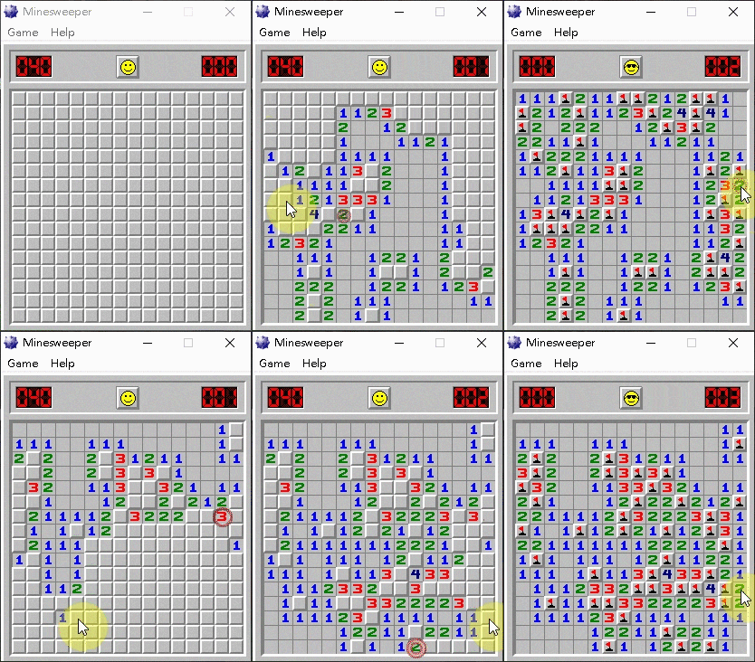
I got addicted to Minesweeper the first few days when I started playing this awesome puzzle game. Solving the game faster every few times gives me great satisfaction of self-fulfillment. However, for the “expert” board setting, where 99 mines are hidden within a 16×30 square grid, I had never obtained a score lower than 100 seconds. Curious of what the fastest solving rate is the one can achieve, I designed a Minesweeper AI program that can automatically play the Windows Minesweeper game.

C language is used for programming, and the algorithm flowchart is displayed in Fig. 1.

Figure 1. Algorithm flowchart of the Minesweeper AI program.

Here breadth-first-search (BFS) is used to search for uncovered squares on the grid, and a queue is used for saving uncovered squares to be analyzed. A game-playing optimized algorithm is written inside the program, and OpenCV is used to take a snapshot of the Minesweeper window region and process the image for subsequent calculations. Mouse movement and click actions are realized by including the windows.h header.

The usage of the program is relatively simple. The user should only execute the Minesweeper game program, and modify the game setting beforehand. After opening the AI .exe file, the program will automatically locate the Minesweeper game, calculate the dimensions, then start playing. If a mine is accidentally clicked, the program will continue to play the next game until a fully uncovered board is achieved.

Here is a clip demonstrating the Minesweeper AI playing an expert level game and winning in 7 seconds. It failed on the first try almost at the end, but succeeded on the second try.

[Download program for the Minesweeper AI (Can only run on a windows 64-bit OS)]

Guess the Number AI

Posted on 2019/09/10 | by andrewlai61616

After completing the first two projects of the Guess the Number series (Guess the Number (Windows) and Guess the Number (iOS)), I made an AI that can play this game at a high-human level.

It has been proven that at most 7 turns are needed to guess the answer, with a best average game length of 5.21 turns. For this game, all the possible combinations (e.g. “0123”, “7381” …) can be saved into a 1D array. After each guess, the possible combinations for the answer will be reduced. Therefore, the algorithm of the program is written for finding a number that will minimize the maximum possible combinations left. The time complexity for each turn is O(n³), and an average of 5 turns of guessing if needed for an arbitrarily chosen number.

For using the program, the user must first choose a 4-digit answer (e.g. “0123”), and input the two numbers [A] and [B] according to the game rules and the numbers guessed by the program. For instance, if the answer is “1357”, and the AI guesses “3127”, the user must input 1 2 ([A] = 1, [B] = 2).

Here’s a demonstration of the AI program guessing the answer “8192” in 5 guesses:

[Download Guess the Number AI program]

[Source code for the Guess the Number AI program]

Nonogram AI

Posted on 2019/09/10 | by andrewlai61616

Nonograms (also known as Picross, Griddlers, Pic-a-Pix, and various other names) are picture logic puzzles, in which the cells in the grid must be colored or left blank according to the numbers on the side of the grid to display hidden pictures.

Figure 1. The initial and complete state of a 25×25 grid Nonogram.
(Source: https://www.nonograms.org/nonograms/i/32344 )

For a classical type of game, the numbers are a form of discrete tomography that measures how many unbroken lines of filled-in squares there are in any given row or column. For example, a clue of “1 2 3” would mean there are sets of one, two, and three filled squares, in that order, with at least one blank square between successive sets.

Solving Nonograms can be very time-consuming, and can be tremendously brain-twisting as the grid size increases, thus I created an AI program for automatically solving these puzzles.

The program utilizes the depth-first search algorithm that runs recursively from the top to bottom row. For the j^th column of the i^th row, the black or blank spaces must satisfy the tomographic rules formed by the numbers of the current row and column. This is a relatively simple approach for calculating the answer. However, because the algorithm does not solve the game using a more intuitive method for solving interrelated constraints, it will use a lot of time for big grids (over 40×40).

For the input format of this program, two numbers indicating the number of rows and columns are given first (n and m). Afterwards, there are n rows of data, with each row k starting with a number n_k indicating how many numbers are given in that row, and followed by n_k numbers representing the discrete tomography of black spaces of that very row; then there are m rows of data, and also starting with a number m_k for the k^th row, and followed by m_k numbers representing the discrete tomography of black spaces for the k^th column.

Here’s an example input for the Nonogram in Fig. 1:

25 25
1 8
2 7 3
1 16
2 11 4
2 13 2
2 14 2
1 18
2 8 4
2 6 4
2 5 5
3 4 2 2
3 4 3 1
3 3 2 1
2 3 2
2 3 2
3 2 1 4
3 2 1 4
3 2 1 4
3 3 1 4
2 5 4
1 11
1 10
1 5
1 5
1 6
1 1
1 2
1 2
1 4
1 11
1 13
1 15
2 9 3
2 8 3
3 7 5 2
3 7 3 4
3 6 2 3
3 8 3 2
2 13 2
2 10 2
3 5 5 3
4 4 1 4 6
4 1 2 2 8
3 3 1 10
4 3 1 4 4
4 2 1 2 3
3 2 1 2
2 2 1
2 2 1
1 1

A demonstration for using the AI program for solving a 39×50 Nonogram in about 22 seconds is shown below. The result displays an owl sitting on a branch (Fig. 2).

Figure 2. The complete state of a 39×50 Nonogram displaying an owl on a branch.

[Download program for the Nonogram solver AI]

[Source code for the Nonogram solver AI]

Othello AI

Posted on 2019/09/10 | by andrewlai61616

Othello (a variant of the traditional game Reversi) is a two-player strategy board game played on an 8×8 square field, where each player takes turns placing black or white pieces and capturing the other player’s pieces.

Figure 1. Othello board game.

The Othello AI program is the second board game AI that I have written in junior high school (the first is the Tic-Tac-Toe AI). Just like the programming strategy for the tic-tac-toe AI, I used the logic thinking experiences that I had learned while playing this game, and hard-coded some summarized strategies into this program.

Compared with the tic-tac-toe AI, which has a game-tree complexity of 9! = 362880, Othello is much more complex, yielding a stunning complexity of approximately 10⁵⁸. This makes the game still mathematically unsolved up to this very day. Therefore, instead of calculating the definite winning strategy, this Othello AI rather tries to find relative advantageous points (e.g. the corners), and moves that will temporarily maximize the number of pieces which it occupies by the coded algorithm, making it a beginner ~ intermediate level AI.

Here is a demonstration of using the Othello AI program:

[Download Othello AI program]

[Source code for the Othello AI program (Visual Basic 6.0 form file)]

Sudoku AI

Posted on 2019/09/10 | by andrewlai61616

Sudoku is a commonly known logic puzzle game, and had been one of my favorite puzzle games.

Having the experience for creating the simple Tic-Tac-Toe AI, I started to take on this challenge for creating an AI that can solve Sudoku.

Figure 1. The initial and complete board state of an expert-level Sudoku game.

I had written this AI program when I was in junior high school using Visual Basic 6.0. Having no prior knowledge for algorithms and data structures (which I learned in senior high school), I came up with a rough version of the backtracking algorithm myself, and implemented it on the AI. Here, the backtracking algorithm is a kind of depth-first search (DFS), and is guaranteed for finding a valid solution. Constraint programming is also integrated with the backtracking algorithm, since it is a very intuitive way for solving the puzzle.

Here is a clip demonstrating the Sudoku Solver program solving a hard-level Sudoku in around 5 seconds:

Here is another one that solved an expert-level Sudoku in around 44 seconds:

[Download program for the Sudoku Solver]

[Source code for the Sudoku Solver (Visual Basic 6.0 form file)]

Gomoku AI

Posted on 2019/09/10 | by andrewlai61616

Although entering a department different from Computer Science (CS), I still had a majority of acquainted people in NTU-CS. One day, a friend of mine who was studying in CS challenged me of making an AI of some board game. The two of us would make AIs of that game and try to win the other one using the AI. Thinking it might be some challenging but interesting subject, I started to make this Gomoku AI.

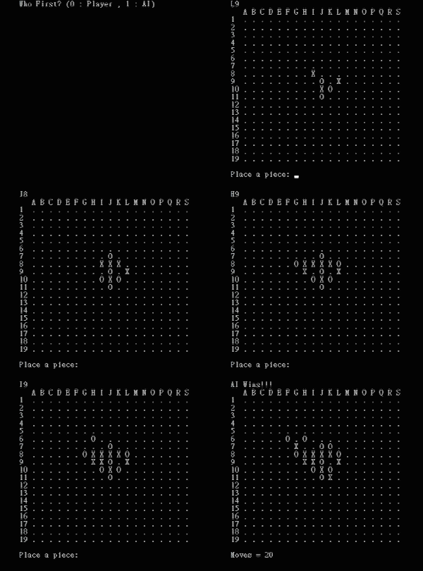
Figure 1. Game playing demonstration of the Gomoku AI program.

Being a board game with so many possible states (more than the Othello AI I had made when I was in junior high school, which only has a 8×8 grid) , it is considered overly time wasting for the AI to traverse all the possible combinations, even just within 10 moves! Game tree graphs, graph traversal algorithms (e.g. DFS, BFS) and optimal searching algorithms (e.g. Alpha–beta pruning, A*) are usually implemented for decreasing computational time and achieving the best strategy. In this project, I only used the depth-first search (DFS) algorithm, along with some hard coded optimization decisions to create this program. Although being able to place a few initial pieces successfully, the program suffers from a large amount of computational time being spent. Most of the time after a few moves, the program will just run for a few hours (or days) before taking the next move, which is obviously very a serious problem for the AI.

Nevertheless, the environment and rules of the Gomoku game engine was successfully constructed, which allowed two players to play against each other. Nowadays, these board game AI are usually designed using deep neural networks, such as AlphaGomoku, an Alpha-Go-based Gomoku AI. Constructing these AIs would be a possible future work for optimizing this game agent.

Tic-Tac-Toe AI

Posted on 2019/09/10 | by andrewlai61616

Artificial intelligence (AI) has long inspired me, and had spurred me on to come up with interesting programs or projects that I had not imagined before. Since great oaks from little acorns grow, this tic-tac-toe AI project is the first and one of the most important programs I have made that can be said to possess artificial intelligence. (~age 15, 2011)

Either with the player playing first or the computer, the AI will never lose! Being a very simple game that one could easily master, tic-tac-toe can yet be quite complex in a way in that there is actually a total of 255168 possible outcomes! Fig. 1 illustrates all the possible board states until the 5^th move using an optimal strategy with the 1^st move at the center (States that can arise from mirroring or rotating the shown states are excluded). The green circled states are those which the circles have won, and the yellow ones are those which the circles will eventually win while continuing to implement the optimal strategy. We can see that it actually gets quite complicated after the 3^rd move.

Figure 1. Possible states of Tic-Tac-Toe until the 5th move starting from the center.

Since back then I knew nothing about algorithms (which I had started to learn at senior high school), I hard coded almost all the conditions using very basic syntax: If…Else…End If and For…Loop. The AI will sometimes move randomly, but it will always follow an optimized strategy. It took me ~650 lines of code and several days of hard work to complete.

This project demonstrated the possibility of programs to achieve human level performance for playing simple games. Although objectively not considered an astonishing one, I was surely amazed and unprecedentedly inspired by the potential of programming algorithms for AI; which further on motivated me to create AI programs of increasing difficulties (refer to Gomoku AI, Sudoku AI, Othello AI, Nonogram AI, Guess the Number AI, Minesweeper AI).

Category: Artificial Intelligence (AI)

Survival Rate Prediction Model for Startup Companies

Reinforcement Learning applied to Forex Trading

Remote Commandable Self-Driving Toy Car

Minesweeper AI

Guess the Number AI

Nonogram AI

Othello AI

Sudoku AI

Gomoku AI

Tic-Tac-Toe AI

Looking for something?