I’m an active person with strong learning abilities, being profoundly inspired by programming when I was young. In junior high school, I self-learned Visual Basic 6.0 for making simple programs and won first prize in science fair competition. In senior high school, I learned C language along with algorithms and data structures, and won 5th ~ 10th place in Taiwan Olympiad in Informatics. These series of events firmly established my outstanding programming skills.
In college, I majored in mechatronics and attained relevant skills for various applications. I teamed up with schoolmates for developing an alarm clock that can awake people using a specific fragrance and earned 40,000NTD in a fundraising event. During this period, I acquired PCB layout skills and the ability for practical usage of microcontrollers, IC chips and different electronic components. I have lots of practical experiences for machine learning and data mining using neural networks (Python + Tensorflow), and won first prize in a competition held by Taiwan Semiconductor Manufacturing Company (Big Data Analytics for Semiconductor Manufacturing). I also have experience in designing digital logic circuits using Verilog and Hspice, and obtained high scores in class.
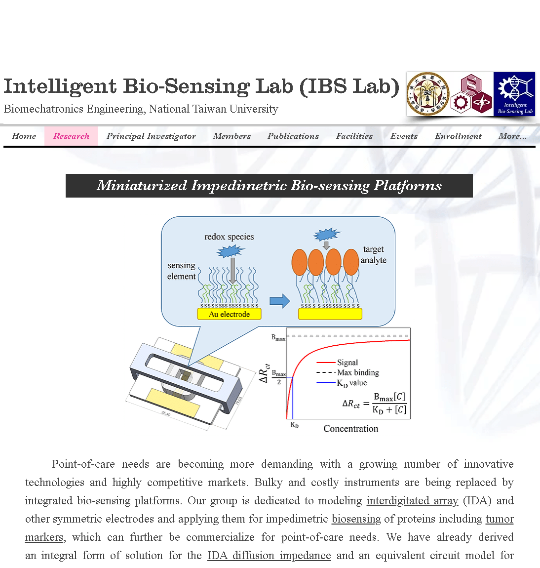
My graduate research topic focuses on interdigitated array electrode chips applied to electrochemical impedimetric biosensing. I learned the complete microfabrication process for microelectrodes and microfluidic chips, utilized Raspberry Pi for developing a wireless and miniaturized website-controlled impedance detection device, and applied those to my own research. Accordingly, I wrote a full research article as first author, and published it on an international journal (Electrochimica Acta, IF = 5.383) (DOI: 10.1016/j.electacta.2019.134629). Now, I currently work as research assistant in my lab, and take the lead in research and development.
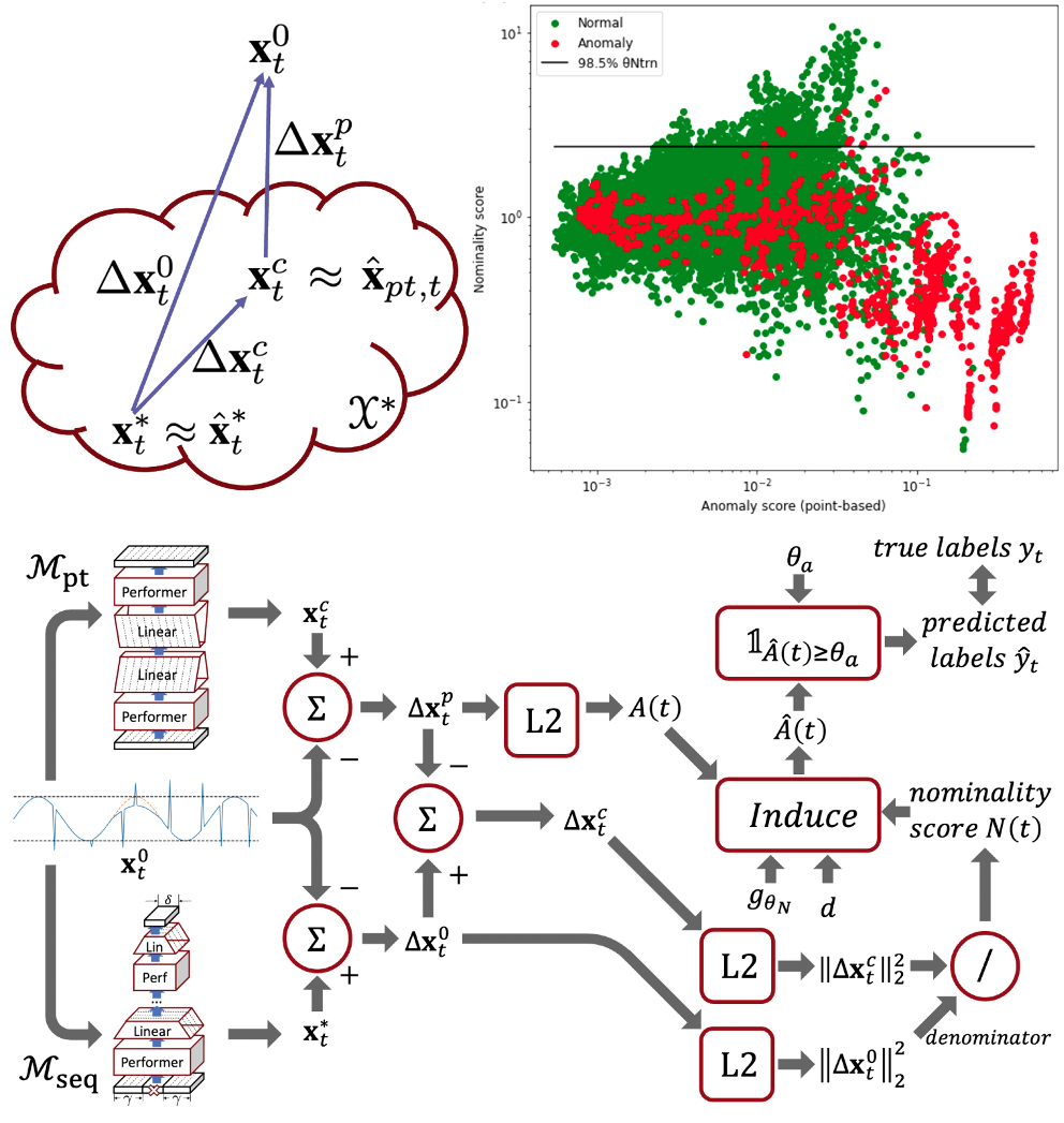
Time series anomaly detection is challenging due to the complexity and variety of patterns that can occur. One major difficulty arises from modeling time-dependent relationships to find contextual anomalies while maintaining detection accuracy for point anomalies. In this paper, we propose a framework for unsupervised time series anomaly detection that utilizes point-based and sequence-based reconstruction models. The point-based model attempts to quantify point anomalies, and the sequence-based model attempts to quantify both point and contextual anomalies. Under the formulation that the observed time point is a two-stage deviated value from a nominal time point, we introduce a nominality score calculated from the ratio of a combined value of the reconstruction errors. We derive an induced anomaly score by further integrating the nominality score and anomaly score, then theoretically prove the superiority of the induced anomaly score over the original anomaly score under certain conditions. Extensive studies conducted on several public datasets show that the proposed framework outperforms most state-of-the-art baselines for time series anomaly detection.
C.-Y. Lai, F.-K. Sun, Z. Gao, J. H. Lang, D. S. Boning, Nominality Score Conditioned Time Series Anomaly Detection by Point/Sequential Reconstruction, Neural Information Processing Systems (NeurIPS), 2023. [arXiv] [NeurIPS] [GitHub]
C.-Y. Lai, F.-K. Sun, J. H. Lang, D. S. Boning, Unsupervised Multivariate Time Series Anomaly Detection for High-Frequency Data, Microsystems Annual Research Conference (MARC), (2023). [proceedings]
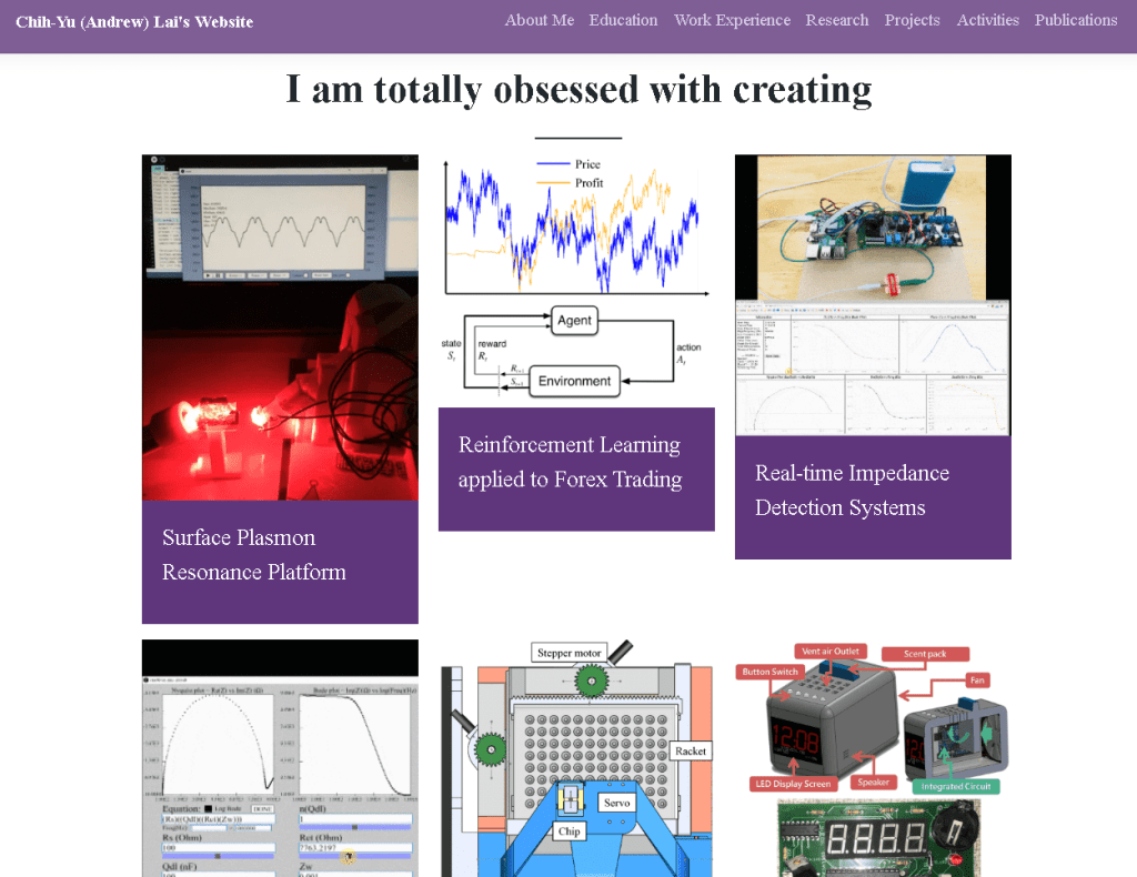
This project is dedicated to investigating the difficult audio-to-video generation with representation learning. Audio-to-video generation is an interesting problem that has abundant application across several industrial fields. Here, we propose a novel training flow consisting of pre-trained models (StyleGAN3, Wav2Vec2, MTCNN networks), newly trained models (variational autoencoders and transformers), and an adversarial learning algorithm. To the best of the author’s knowledge, this is the first implementation of audio-to-video generation using a pre-trained StyleGAN3. The input is a speech audio sequence and an image of a face. Our model will learn to “animate” the face by predicting facial expressions and lip movements. We find that the latent code of our generative model can be encoded 16-fold into a 96-dim vector that retains the information of the talking face. By using this method, audio-to-video generation can be realized without training any generative models, and only latent codes should be predicted from audio. This minimizes our requirement for dataset size and training time. (The reconstructed videos can be found here.)
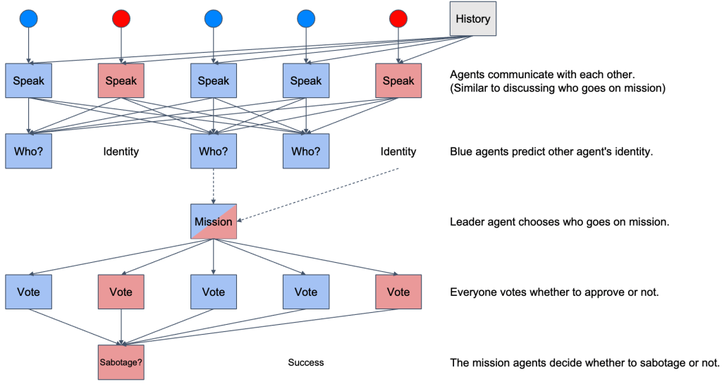
We trained proximal policy optimization (PPO) agents to play the hidden role game The Resistance. Learning whether or not other actors are behaving in your interest, or only pretending to, is a problem widely unstudied in reinforcement learning. We allow the agents to create and develop their own form of communication which allows them to adversarially influence the actions of other agents. We develop several baseline strategies and metrics to evaluate and quantify our training results. A total of 10 models are constructed and used for completing different tasks during the game by two competing teams. We found that the PPO agents can play competitively against our baseline strategies, without training on these baselines. This means the agents not only learn to play against their non-stationary counterparts but learn generic strategies to play against unknown players. Our experimental results show that the agents developed communication in order to identify each other’s roles, resulting in an increase in their win rates. Therefore, we’ve shown that emergent communication is helpful for cooperative and adversarial multi-agent reinforcement learning when there are partially observable states.
Lyto Different Color is a color differentiation game on Facebook. Each level, there are NxN circles on a board, with one circle having a color slightly different from all the others. The player must find the circle with different color and click on it in order to go to the next level. During the early stage of the game, the difference between the color of the unique circle and the color of the other circles gets smaller, and N gets larger, making it become more difficult. For most people, level 50 is considered a high score, and it is almost impossible for a normal human to reach level 100.
I simply wanted to break this limit, so I wrote a Python script for continuously taking a snapshot of the section of the game screen, find the circles, reading their color, and pressing on the circle with unique color. It is comparatively easy for the AI to recognize the differences, since it reads the colors as an RGB value, where any difference in the values represents a difference in color.
Python Imaging Library (PIL) is used for capturing the game screen, which approximate takes a screenshot every 0.7 seconds. Afterwards, the boundary of the circles is found by finding pixels that have a different color compared with the plain background color. Then, N is found by counting continuous blocks of identical colors from a 1D diagonal slice of array from the top-left to bottom-right corner of the boundary. By finding these values, the center of every circle can be located, which the program retrieves the colors from and compare them. At last, the circle with unique color is found, and the program sends a signal to the mouse for pressing on the target position. Fig. 1 illustrates a graphical description of the program algorithm.
Figure 1. Graphical description of the algorithm for Lyto Different Color AI.
Here’s a clip of the program playing the game (2x speed):
I started to self-learn programming from the age of 13. Back then, I used Visual Basic for designing simple games and applications. Having the ability to create, I opened a world full of amazement. Not only did more and more ideas came to me, I actually relatively improved my logic thinking and mathematics. I started to use C language and app designing for developing projects from the age of 15. Here are some of the simple games and programs which I have made in my leisure time.
It’s not just about the grades. Mostly, it’s about the inspiration, the potential of knowledge that deeply impresses. I have individually and cooperatively created several projects in school. Here are some mini projects that have once motivated me to keep on exploring and discovering.
After being approved for entering my department (NTU BIME) in university, I joined the graduation ceremony group in my high school (HSNU).
I act as one leader among the three leaders in the network group. The objective of this group is to construct the graduation ceremony website.
My main responsibility is to collect information from other groups (e.g. public relationship group, ceremony group…) and to organize them, where the other two leaders use these data to construct the website.
In my view, this is by far the website with the most abundant resources and exquisite design among all other graduation ceremony websites in our high school.
Figure 1. A snapshot of the graduation ceremony website.
Intelligent Bio-Sensing Lab Website
After graduating from graduate school in NTU, I worked as research assistant in my lab (intelligent bio-sensing lab, IBSLAB) led by professor Lin-Chi-Chen. During this period, I constructed the lab website using Wix.
For webpage design, HTML, CSS, JavaScript and PHP are used as the coding language; jQuery is used for Ajax calling; Masonry is used for grid layout display; MathJax is used for equation expressions; and other additional plugins are installed for realizing several features.
The approach for using surface plasmon resonance (SPR) as an optical method for detection of biomolecules with low concentration in real-time has been widely investigated. However, such instruments are highly expensive and bulky, hindering development for portable devices. After discussing with my professor Dr. Lin-Chi Chen about this project, I developed a simple and preliminary platform that can measure the refractive index change of a liquid using SPR.
Figure 1. Prism-based SPR detection
The prism-based SPR system (Fig. 1) is widely used in practical applications, including today’s instruments. Here, A p-polarized light source is refracted into a prism, totally internal reflected (TIR) on another side, and refracted out at another, being received by a light detector. Usually a fluid channel with a special treated surface (e.g. glass with evaporated Au) is placed on the top where the TIR effect happens.
Figure 2. Attenuated total reflection phenomenon (ATR).
When the light beam enters at a certain incidence angle, surface plasmon polaritons can be excited in a resonant manner at the TIR interface. This means there would be attenuated total reflectance (ATR) phenomenon at that angle, and a decrease of light intensity would exist (Fig. 2). This incidence angle is called the SPR angle, and has a linear relationship with the reflection index of the fluid-glass interface.
Hardware Design
Figure 3. Materials used in this project.
The materials used for constructing this platform are in Fig. 3. As the light emits from the laser, it passes through the convex lens to change its direction, ending up in a slightly diverging beam, entering the prism and hitting the chip surface at different incidence angles (Fig. 4).
Figure 4. Simulation of red light from a laser passing through a convex lens, a prism, and through a microfluidic chip.
The range of incidence angle (Θ) is calculated so that 62.294° < Θ < 72.203°, which at some value within this range there exists the SPR angle of water. Fig. 5 shows a few important specifications for the setup.
Figure 5. Specifications for materials using in this project.
Here’s a clip of the SPR phenomenon appearing at the upper region of the reflected light after an Au-evaporated glass slide is dropped with deionized water.
For detection of light signal, a photoresistor is fixed on a linear gear of the light detector holder. The position of the gear is controlled by a stepper motor fixed on the holder (Fig. 6). The totally internal reflected light will be captured by the moving photoresistor for recording light intensity at a certain position.
Figure 6. Light detection module consisting of a photoresistor, a linear gear, a stepper motor, and a 3D-printed holder.
Program Control and User Interface
Arduino is used for controlling the stepper motor and reading the output of the photoresistor. Prior to reading, the resistances are converted to voltage signals using a simple circuit. For developing a program with visual UI, processing language is used for communicating with Arduino. Fig. 7 shows the program consisting of a signal display panel and several buttons for different functions.
Here’s a demonstration of using the combined UI and hardware platform:
The program will record light intensity, and convert it to a signal with a range between 0 and 1000. In order to calculate the differential signal (the signal with SPR phenomenon minus the signal without SPR phenomenon), the program will average the signal being detected at a certain position within every cycle. By deleting the two averaged signals, this differential signal can be calculated. The differential can indicate the position that the ATR occurred.
Below is another clip for SPR detection using a microfluidic chip, the ATR can be clearly detected by the platform.
The direction of the speed of the linear gear will also have an impact on the signal. In Fig. 8, a smoother SPR curve (average difference of ΔV) is calculated by averaging the data obtained by the clockwise and counter-clockwise direction.
Figure 8. SPR Differential signal of light intensity converted to voltage including clockwise and counter-clockwise directions.
The total cost is a few thousand NTD, which is very low compared with commercial instruments (~1 million NTD). In the future, I hope that this platform can be reinforced for detecting bio-samples in real-time.
The minimization of instruments and relevant devices for data acquisition is a major demand for portable bio-sensing systems. In the following paragraphs, the development of real-time impedance detection systems is detailed, where generations α and β are developed. Generation α serves as the proof-of-concept for the construction of a detection system that can measure impedance from 0.1 to 10000 Hz. Generation β improves several features of generation α, such as the applied frequency range, measured impedance range, detection time, and detection repeatability. In generation β, a website is constructed for controlling the system and acquiring real-time data so that any remote user can have access using smart devices without the need for installing any apps or services. This is particularly useful regarding portability and accessibility, which is highly competitive for integrated biosensors concerning the internet of things (IoT) technologies.
Scheme for Generation α
The general scheme for this generation is depicted in Fig. 1. A function generator is used for producing sine voltage waves across a symmetric electrode system, then a NIDAQ device (USB-6210) is used for collecting voltage signals from the measurement circuit. The signal is processed and sent to a computer for data analysis and plotting.
Figure 1. General scheme for real-time impedimetric detection system (generation α).
Data Analysis using LabVIEW for Generation α
The block diagram and front panel of the LabVIEW data analysis procedure are depicted in Fig. 2. Two signals are acquired by the DAQ device: the input voltage and the amplified current (measured in voltages) of the electrode chip. When the amplification ratio of the current is known, the current can be calculated by dividing the measured voltage with the known ratio. The frequency is calculated using Fourier transform of the signals. The absolute impedance (|Z|) is calculated by dividing the amplitude of the input voltage by the current. The phase angle can be found by calculating the phase difference between the two signals. These two values are plotted on the graph in the front panel and can be saved as comma-separated values (.csv) that can be used for data fitting.
Figure 2. (a) Control panel and (b) block diagram for impedance measurement of Z_GENα using DAQ device and LabVIEW software.
Figure 3. A photo of the whole system of generation α.
The clip below shows real-time impedance measurement using generation α. A microfluidic interdigitated array (IDA) chip (wg/we = 25/100μm, where we is the electrode bandwidth and wg is the gap width) is used. The flow rate is 0.1μL/s and the applied frequency is 100Hz.
A major difference between the detection of phase angle of generation β and that of generation α is that the former always output a sinusoidal wave from a phase angle of 0°, while the latter outputs from an arbitrary angle. By recording the time of the start of detection, the phase angle can be obtained by only measuring the output current wave. For instance, if the peak of a current wave is detected at the start of detection, then it can be deduced that the phase angle is -90° (Fig. 4).
Figure 4. A current wave of phase angle -90°.
In this generation, a miniaturized, portable, real-time, low-cost and remote commandable (website-based) system is developed. The target set for it has a whole list of goals in addition to the main features of a typical impedance analyzer: miniaturization, portable, real-time, low-cost and user-friendly. For the hardware, a Raspberry Pi 3 b+ model, an impedance measurement circuit, and a microelectrode sensor chip are integrated. The scheme of generation β is illustrated in Fig. 5.
Figure 5. General scheme for real-time impedimetric detection system (generation β).
Impedance Measurement Circuit Design
For generation β, several IC chips are integrated on a universal PCB board for achieving the functions of the function generator and the DAQ device in generation α. The AD9833 waveform generator is used for the production of sinusoidal voltage waves. TL074op-amps are used for transformation of electric signals. The fast precision op-amp OP42 is used for amplification of the small signal current running through the sensor chip. A voltage stabilizer module made from UA741 op-amp is used for providing stable voltage signal. The analog-to-digital converterAD7822 is used for signal acquisition, and sending digital signals to Raspberry Pi (Fig. 6).
Figure 6. Circuit schematic for generation β.
Data Processing
The raw signal obtained by the ADC is an 8-bit resolution data ranging from 0 to 255 at a rate of 1MS/s (mega samples per second). Due to the relatively fast sampling speed by Raspberry Pi and some imperfections within the circuitry, there may appear to be some defects or noisy signal in the acquired data. Thus, a strategy for data processing before the calculation of |Z| and phase of the measured system is designed. The general concept is depicted in Fig. 7 for a raw signal with a linearly transformed value between 0 and 1.
Figure 7. Strategy for impedance range detection and data processing for generation β.
First, leading and ending consecutive zeros are trimmed, and the data is shifted to a start of a non-zero value. Second, values outside n standard deviations from the average of m data points are removed where n and m are arbitrarily defined constants for a specific sampling frequency. Third, the removed values are linearly bridged between non-removed values to form continuous data points. Fourth, smoothing is performed by averaging k data points to form a new value. |Z| is found by calculating the standard deviation of the overall data which equals the zero-mean root-mean square (RMS) of the signal and is proportional to the amplitude with a relationship of . The phase is obtained by first calculating the average of the remainder of the time (μs) of a data point, which is larger than or equals the mean and its previous data point is smaller than the mean, divided by the number of data points within a repeating sine wave cycle, then linearly transforming it to a value between 0 and 360 degrees.
Website Server
For portable devices dedicated to point-of-care applications, a miniaturized device must be set up that contains user-friendly interfaces and well-designed data display graphics. A smart phone might come in handy when it comes to the such integration. Applications using smart phone for electrochemical on-chip detection of biomarkers are presented and published every year. For the above reasons, a website platform for the user interface of generation β is set as a target for its improvement compared with generation α, which can be accessed using local networking on either a personal computer, a smart phone, a pad … etc. The overall structure is shown in Fig. 8.
Figure 8. Structure of the web server of generation β.
Results for Generation β
The photograph of generation β is shown in Fig. 9. The dimension is 22(L)×10(W)×6(H) cm3, which makes it a portable system. The Raspberry Pi controls the circuitry by sending voltage signals towards the IC chips. The sinusoidal current passes through the sensor chip, gets amplified, then is sampled by the ADC. The transformed digital values are read by the Raspberry Pi and being processed. At last, impedance values are plotted on the website.
Figure 9. Photograph of generation β.
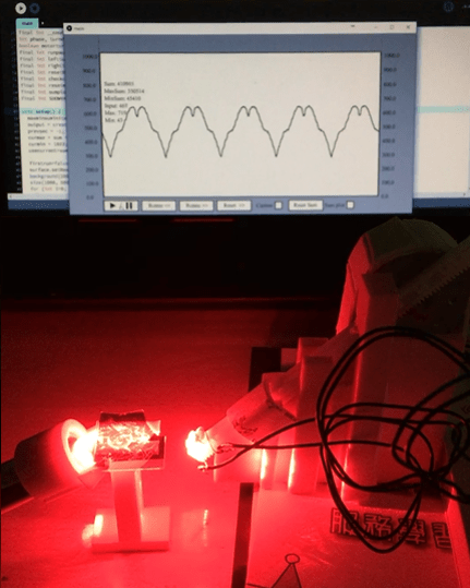
The content below is a clip for demonstration of using the website interface of generation β. The website shows |Z| vs f, phase vs f, Im(Z) vs Re(Z), Re(Z) vs f and –Im(Z) vs f at the same time. The collected data can be saved to a CSV file for further analysis.
A mobile power supply can be simultaneously used as the power supply for the circuitry and Raspberry Pi (Fig. 10), and smartphone-controlled impedance detection can also be achieved (also shown in clip below).
Figure 10. Generation β powered by a power bank.
Microfluidic Impedimetric Detection using Interdigitated Au Electrode Chip
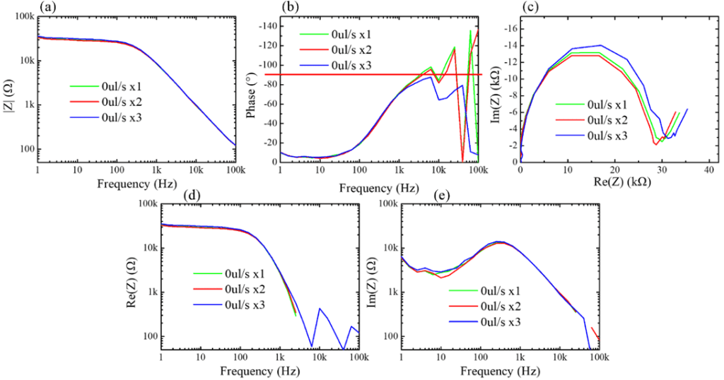
The repeatability of electrochemical impedance spectroscopy (EIS) detection in a microfluidic interdigitated array (IDA) chip system is tested using generation β as the measuring system. In Fig. 11, it can be seen that a fairly stable measurement of |Z| can be achieved within a frequency range of 1 ~ 105Hz, and an absolute impedance range of about 0.1 ~ 30kΩ can be detected. However, at high frequencies, the phase angle does not have a reasonable and repeatable value. This reason is due to the larger noise of sampling values at high frequencies. A red line is drawn at 90° on the phase vs f plot. Normally, phase angles wouldn’t exceed this value because that would give rise to a negative Re(Z), and does not correspond to any familiar electrochemical mechanism. Such sampling errors and data processing are needed to be improved.
Figure 11. (a) |Z| vs f, (b) phase vs f, (c) Im(Z) vs Re(Z), (d) Re(Z) vs f and (e) Im(Z) vs f for single EIS detection of IDA chip at 0μL/s flow speed using generation β. The channel width is 0.5mm. Vamp = 50mV. Running buffer: 5mM Fe(CN)63-/4-in PBS.
My research as a graduate student focuses on biosensing applications using electrochemical impedimetric methods. Unlike mechatronic systems, these applications consider a dynamic environment at such a microscale, it is quite hard to perceive what is really going on when we merely recognize the change of physical property. I usually ask myself: What is the underlying mechanism? Tucked away from the limit of horizon of the human eye, we often see nothing happening when doing these experiments.
The result of task 1 supports the hypotheses of task 2 and 3.
Physical Environment Setting
The simulation environment is set as the interior of a microfluidic channel with gold microelectrodes. See the film below for visualization.
The chip is fabricated using soft lithography and photolithography. The microfluidic channel has a width of 1mm and a height of 100μm at the center. The gold microelectrodes form a pair for square pads (300×300μm) at the center of the channel (Fig. 1).
Figure 1. Microfabrication process, dimensions, and microscopic view of the microfluidic electrode chip used in this project.
Velocity Field Simulation Inside Microfluidic Channel
The objective of this task is to simulate the fluid velocity field inside the channel on a sliced plane. Due to the fact that 3D simulation is time-consuming, if a 3D environment can be reduced to a 2D environment, then a large amount of time can be saved. By performing this task, it can be seen if dimension reduction modeling of task 2 and 3 are feasible.
Considering the physical nature of the microfluidic channel, a laminar flow model is implemented along with the Navier-Stokes equation:
, which means a balance between inertia (\(\rho(\textbf{u}\cdot\nabla)\textbf{u}\)), pressure (\(-pI\)), viscous (\(\mu(\nabla \textbf{u}+(\nabla \textbf{u})^T)\)) and external (\(F\)) forces. A stationary study is implemented (\(\rho \nabla \cdot \textbf{u}=0\)), and water is set as the fluid.
Fig. 2 shows the 3D velocity field inside the channel. A bigger arrow indicates a larger velocity magnitude. The reason that the velocity is faster at the center is because of the lower channel height.
Figure 2. 3D velocity field inside microfluidic channel.
Fig. 3 shows animated 2D velocity fields of sliced planes inside the channel. Due to laminar flow, velocities near the boundary get close to zero. However, the steady-state velocity reaches a constant value away from the boundary.
Figure 3. 2D velocity fields for xy and zy sliced planes.
A top view of the velocity field and the velocity at different x positions are shown in Fig. 4. It can be concluded that at the center of the channel where the microelectrodes lie, the fluid velocity stays constant, and subsequent tasks can be carried out using 2D models.
Figure 4. Top-view and x position-dependent velocity magnitude of fluid.
Real-time Molecule Immobilization on Gold Surface.
For microfluidic electrochemical biosensors, it is quite common that immobilization of sensing elements takes place at the center of the channel on electrode surfaces (e.g. Au). In this task, molecules are simulated to flow past the channel, and be immobilized on the electrode pad at the bottom center. A slice on the zy plane is used as the modeling geometry of this task (Fig. 5).
Figure 5. Modeling geometry used in task 2. A sliced area of the microfluidic channel with pad electrode at the bottom center is used.
Here, the molecules convect and diffuse near the surface, the rate of immobilization is determined by several factors including the inlet concentration (c0), diffusion coefficient (D), maximum surface molecule density (Γs). The convection-diffusion equation and transport-adsorption equation are used along with time-dependent study:
$${{\partial c} \over {\partial t}} + \nabla \cdot (-D\nabla c) + \textbf{u} \cdot \nabla c = R$$
For the transport-adsorption equation, it is assumed that the change of surface concentration plus the rate of surface diffusion equals the rate of Langmuir adsorption isotherm.
Fig. 6 shows the time-dependent surface concentration (cs) change when c0 = 1μM, and Fig. 7 shows the binding curve (probe density vs time) for different values of c0.
Figure 6. Time-dependent surface concentration (cs) change. t = 0~18hr.
Figure 7. Probe surface density (molecules/cm2) vs time (hr).
At concentrations above 0.1μM, the probe density almost saturates to a value of 9.6×10¹² molecules/cm2 before immobilizing for 10 hours. The result highly resembles a typical binding curve, suggesting the possibility for computer simulating assisted optimization of in vitro parameters, which is really helpful for understanding underlying mechanisms for the system.
EIS is a rapid and label-free method for detection of bio-molecules, and is widely implemented on a variety of biosensors. In this task, I simulated EIS diagrams by changing the values of the heterogeneous rate constant (k0) and the double layer capacitance (Cdl). Both Cdl and k0 are affected by the immobilized surface molecule density on an electrode surface, and are important physical properties when analyzing EIS data. A slice on the xy plane is used as the modeling geometry of this task (Fig. 8).
Figure 8. Geometry being simulated for task 3. A 2D plane is sliced in the xy direction.
Here, a sinusoidal voltage wave is applied between the two electrodes (amplitude ≅ 5mV), and Bode plots and Nyquist plots can be drawn according to the measured impedance. According to the surface redox reaction, an equivalent circuit can be constructed. The equivalent circuit for this task is shown in Fig. 9.
Figure 9. Equivalent circuit used in my research and task 3.
EIS plots are simulated for different values of k0 and Cdl (Fig. 10).
Figure 10. Bode and Nyquist plots for the simulated EIS data. k0 has a range from 0.001 to 0.1 (cm/s), and Cdl has a range from 0.01 to 100 (uF/cm2).
By undergoing this simulation project, I furthermore understood some fundamental interactions between the physical properties and outcome of my research to a new depth, and developed new concepts about how to improve it.