Electrochemical and Biological Simulation for Microfluidics

My research as a graduate student focuses on biosensing applications using electrochemical impedimetric methods. Unlike mechatronic systems, these applications consider a dynamic environment at such a microscale, it is quite hard to perceive what is really going on when we merely recognize the change of physical property. I usually ask myself: What is the underlying mechanism? Tucked away from the limit of horizon of the human eye, we often see nothing happening when doing these experiments.

That is why simulation is so important! In this project, I performed 3 simulation tasks in order to visualize the changes of important physical properties for my study (impedimetric microfluidic chip for biosensing) using COMSOL Multiphysics.

The tasks are:

  1. Velocity field simulation inside microfluidic channel.
  2. Real-time molecule immobilization on gold surface.
  3. Electrochemical impedance spectroscopy (EIS) simulation.

The result of task 1 supports the hypotheses of task 2 and 3.

Physical Environment Setting

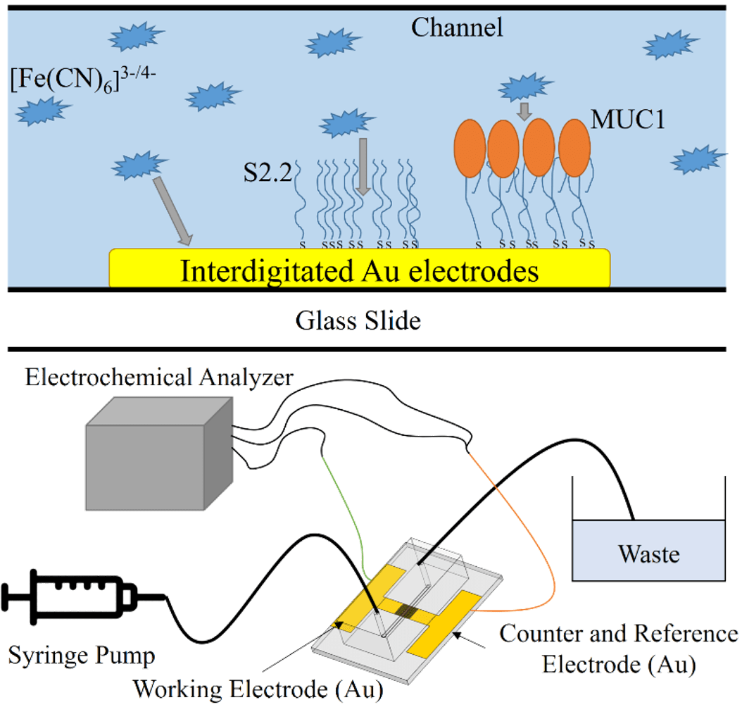
The simulation environment is set as the interior of a microfluidic channel with gold microelectrodes. See the film below for visualization.

The chip is fabricated using soft lithography and photolithography. The microfluidic channel has a width of 1mm and a height of 100μm at the center. The gold microelectrodes form a pair for square pads (300×300μm) at the center of the channel (Fig. 1).

Figure 1. Microfabrication process, dimensions, and microscopic view of the microfluidic electrode chip used in this project.

Velocity Field Simulation Inside Microfluidic Channel

The objective of this task is to simulate the fluid velocity field inside the channel on a sliced plane. Due to the fact that 3D simulation is time-consuming, if a 3D environment can be reduced to a 2D environment, then a large amount of time can be saved. By performing this task, it can be seen if dimension reduction modeling of task 2 and 3 are feasible.

Considering the physical nature of the microfluidic channel, a laminar flow model is implemented along with the Navier-Stokes equation:

$$\rho(\textbf{u}\cdot\nabla)\textbf{u}=\nabla\cdot[-pI+\mu(\nabla \textbf{u}+(\nabla \textbf{u})^T)]+F$$

, which means a balance between inertia (\(\rho(\textbf{u}\cdot\nabla)\textbf{u}\)), pressure (\(-pI\)), viscous (\(\mu(\nabla \textbf{u}+(\nabla \textbf{u})^T)\)) and external (\(F\)) forces. A stationary study is implemented (\(\rho \nabla \cdot \textbf{u}=0\)), and water is set as the fluid.

Fig. 2 shows the 3D velocity field inside the channel. A bigger arrow indicates a larger velocity magnitude. The reason that the velocity is faster at the center is because of the lower channel height.

Figure 2. 3D velocity field inside microfluidic channel.

Fig. 3 shows animated 2D velocity fields of sliced planes inside the channel. Due to laminar flow, velocities near the boundary get close to zero. However, the steady-state velocity reaches a constant value away from the boundary.

Figure 3. 2D velocity fields for xy and zy sliced planes.

A top view of the velocity field and the velocity at different x positions are shown in Fig. 4. It can be concluded that at the center of the channel where the microelectrodes lie, the fluid velocity stays constant, and subsequent tasks can be carried out using 2D models.

Figure 4. Top-view and x position-dependent velocity magnitude of fluid.

Real-time Molecule Immobilization on Gold Surface.

For microfluidic electrochemical biosensors, it is quite common that immobilization of sensing elements takes place at the center of the channel on electrode surfaces (e.g. Au). In this task, molecules are simulated to flow past the channel, and be immobilized on the electrode pad at the bottom center. A slice on the zy plane is used as the modeling geometry of this task (Fig. 5).

Figure 5. Modeling geometry used in task 2. A sliced area of the microfluidic channel with pad electrode at the bottom center is used.

Here, the molecules convect and diffuse near the surface, the rate of immobilization is determined by several factors including the inlet concentration (c0), diffusion coefficient (D), maximum surface molecule density (Γs). The convection-diffusion equation and transport-adsorption equation are used along with time-dependent study:

$${{\partial c} \over {\partial t}} + \nabla \cdot (-D\nabla c) + \textbf{u} \cdot \nabla c = R$$

$${{\partial c_s} \over {\partial t}} + \nabla \cdot (-D\nabla c_s) = k_{ads} c(\Gamma_s – c_s)-k_{des} c_s$$

For the transport-adsorption equation, it is assumed that the change of surface concentration plus the rate of surface diffusion equals the rate of Langmuir adsorption isotherm.

Fig. 6 shows the time-dependent surface concentration (cs) change when c0 = 1μM, and Fig. 7 shows the binding curve (probe density vs time) for different values of c0.

Figure 6. Time-dependent surface concentration (cs) change. t = 0~18hr.

Figure 7. Probe surface density (molecules/cm2) vs time (hr).

At concentrations above 0.1μM, the probe density almost saturates to a value of 9.6×10¹² molecules/cm2 before immobilizing for 10 hours. The result highly resembles a typical binding curve, suggesting the possibility for computer simulating assisted optimization of in vitro parameters, which is really helpful for understanding underlying mechanisms for the system.

Electrochemical Impedance Spectroscopy (EIS) Simulation.

EIS is a rapid and label-free method for detection of bio-molecules, and is widely implemented on a variety of biosensors. In this task, I simulated EIS diagrams by changing the values of the heterogeneous rate constant (k0) and the double layer capacitance (Cdl). Both Cdl and k0 are affected by the immobilized surface molecule density on an electrode surface, and are important physical properties when analyzing EIS data. A slice on the xy plane is used as the modeling geometry of this task (Fig. 8).

Figure 8. Geometry being simulated for task 3. A 2D plane is sliced in the xy direction.

Here, a sinusoidal voltage wave is applied between the two electrodes (amplitude ≅ 5mV), and Bode plots and Nyquist plots can be drawn according to the measured impedance. According to the surface redox reaction, an equivalent circuit can be constructed. The equivalent circuit for this task is shown in Fig. 9.

Figure 9. Equivalent circuit used in my research and task 3.

Fick’s 2nd law and Butler-Volmer equation are used for simulation:

$${{\partial c}\over{\partial t}} = \nabla \cdot (D\nabla c)$$

$$j = nFk_0 (c_{Red} e^{ {(n-\alpha_c)F\eta} \over {RT} } – c_{Ox} e^{ {-\alpha_c F\eta} \over {RT} })$$

EIS plots are simulated for different values of k0 and Cdl (Fig. 10).

Figure 10. Bode and Nyquist plots for the simulated EIS data. k0 has a range from 0.001 to 0.1 (cm/s), and Cdl has a range from 0.01 to 100 (uF/cm2).

By undergoing this simulation project, I furthermore understood some fundamental interactions between the physical properties and outcome of my research to a new depth, and developed new concepts about how to improve it.

After completing this project, I also used COMSOL for simulating time-dependent concentration gradient variation of redox molecules in my 1st author journal paper “Diffusion impedance modeling for interdigitated array electrodes by conformal mapping and cylindrical finite length approximation”.

[Full report for this project]

Reinforcement Learning applied to Forex Trading

It is already well-known that in 2016, the computer program AlphaGo became the first Go AI to beat a world champion Go player in a five-game match. AlphaGo utilizes a combination of reinforcement learning and Monte Carlo tree search algorithm, enabling it to play against itself and for self-training. This no doubt inspired numerous people around the world, including me. After constructing the automated forex trading system, I decided to implement reinforcement learning for the trading model and acquire real-time self-adaptive ability to the forex environment.

Environment Setup

The model runs on a Windows 10 OS (i9-9900K CPU) with DDR4 2666MHz 16G RAM and NVIDIA GeForce RTX 2060 GPU. Tensorflow is used for constructing the artificial neural network (ANN), and a multilayer perceptron (MLP) is used. The code is modified from the Frozen-Lake example of reinforcement learning using Q-Networks. The model training process follows the Q-learning algorithm (off-policy TD control), which is illustrated in Fig. 1.

Figure 1. Algorithm for Q-learning and the agent-environment interaction in a Markov decision process (MDP) [1].

For each step, the agent first observes the current state, feeds the state values into the MLP and outputs an action that is estimated to attain the highest reward, performs that action on the environment, and fetches the true reward for correcting its parameters. The agent follows the epsilon-greedy policy (ε = 0.1) for striking a balance between exploration and exploitation.

State, Action and Reward

For the 1st generation, price values at certain time points and technical indicators are used for constructing the states. The technical indicators used are the exponential moving average (EMA) and Bollinger bands (N=20, k=2), and time frames of 1, 5 and 15min are used with the last 10 time points being recorded. A total number of 36 inputs are connected to the MLP.

There are three action values for the agent: buy, sell and do nothing. The action being taken by the agent is determined by the corresponding three outputs of the MLP, where sigmoid activation functions are used for mapping the outputs to a value range of 0 ~ 1, representing the probability of the agent taking that action.

For the reward function, the difference between the trade price (the price when a buy/sell action is taken) and the averaged future price is considered. If a buy action is taken, then the reward function is calculated by subtracting the averaged future price with the trade price; if a sell action is taken then the reward is calculated the other way around. For “do nothing” actions, the reward is 0. A spread is subtracted from the reward for buy/sell actions to obtain the final reward. This prevents the agent to perform actions that result in insignificant profit, which would likely lead to a loss for real trades (Fig. 2).

Figure 2. Reward calculation method for buy/sell actions.

Noisy Sine Function Test

For preliminary verification of effectiveness for the training model and methods, a noisy sine wave is generated with Brownian motion of offset and distortion in frequency. This means at a certain time point (min), the price is determined by the following equation:

$$P(t)=P_{bias} + P_{amp} sin{2\pi \over T}t+P_{noise}$$

where Pbias is an offset value with Brownian motion, Pamp is the price vibration amplitude, T is the period with fluctuating values, and Pnoise is the noise of the price with randomly generated values. (Note that the “price” mentioned here is defined as the exchange rate between two currencies)

Fig. 3 shows a randomly generated price vs time sequence within a range of 50,000 minutes with an initial values Pbias = 1.0, T = 120 min, Pamp = 0.005, and Pnoise amplitude = 0.001. Generally, the price seems to fluctuate randomly with no obvious highs or lows. However, if it is viewed close-up, waves with clear highs and lows can be observed (Fig. 4).

Figure 3. Price vs time of the noisy sine wave from 0 to 50,000 min.

Figure 4. Price vs time of the noisy sine wave from 20000 to 20600 min.

The whole time period is 1,000,000 min (approximately 700 days, or 2 years). Initially, a random time period is set for the environment. Every time the agent takes an action, there is a certain chance (= 1%) that the time will jump to another random point within the whole period. Otherwise, the time will move on to a random point which is around 1 ~ 2 day(s) in the future. This setting is expected to correspond to real conditions, where a profitable strategy can have stable earnings and can also adapt quickly to rapid changing environments.

Fig. 5 plots the cumulative profit for trading using the noisy sine wave signal for 50,000 steps. Although it took approximately 25,000 steps to make the model get “on track”, I recognize this result as an important start for implementing real data.

Figure 5. Cumulative profit from trading using a noisy sine wave signal.

Fundamental Analysis for Economic Events

Fundamental analysis is a tricky part in forex trading, since economic events not only correlate with each other, but also might have opposite effects on the price at different conditions. In this project, I extracted the events that are considered significant, and contain previous, forecast and actual values for analysis. Data from 14 countries of the past 10 years are downloaded and columns with incomplete values are abandoned, making a complete table of economic events.

Because different events have different impacts on forex, the price change after the occurrence of an event is monitored, and a correlation between each event and the seven major pairs (commodity pairs). Table 1 displays a portion of the correlation table for different economic events. The values are positive, which indicates the significance of an event on the currency pair. Here, a pair is denoted by the currency other than the USD (e.g. USD/JPY is denoted as JPY).

Table 1. Correlation table between 14 events and 5 currency pairs. Here, a pair is abbreviated as the currency other than the USD.

Country Economic Event (Index)AUDCADEURGBPJPY
AUDCommodity Prices0.00313 0.00268 0.00266 0.00339 0.00278
AUDMI Inflation Expectations0.003380.001680.002170.002000.00266
AUDRBA Interest Rate Decision0.004280.002620.002580.002980.00225
EURManufacturing PMI0.003310.002840.002630.002980.00278
EURItalian CPI0.003150.003190.002950.003160.00255
EURServices PMI0.003410.002900.002930.002950.00284
EURCPI0.003040.002940.002620.003170.00241
EURGerman Unemployment Rate 0.003150.003150.002730.003130.00246
EURECB President Trichet Speaks0.003440.002480.003410.003020.00268
EURGerman Unemployment Change 0.003130.003130.002680.003070.00243
EURGerman Trade Balance0.003060.002550.003000.002840.00268
EURGerman Factory Orders0.002920.002650.003120.002800.00275
EURGerman Retail Sales0.003040.003040.003530.003100.00275
EURFrench Trade Balance0.003120.003120.002960.003010.00299

A total of 983 events are analyzed. However, due to the fact that a large portion of events have little influence on the price, only 125 events that have a relatively significant impact are selected as the inputs of the MLP.

Real Data Implementation Results

Per-minute exchange rate data of the seven currency pair is downloaded from histdata.com. A period from 2010 to 2019 is extracted, and blank values are filled by interpolation. This gives us a total of approximately 23 million records of price data (note that weekends have no forex data records), and is deemed sufficient for model training. The data is integrated into a table, and technical indices are calculated using ta, a technical analysis library for Python built on Pandas and Numpy.

Figure 6. EUR/USD exchange rate from 2010 to 2019.

Summing the inputs from technical analysis, fundamental analysis, and pure price data, a total of 1049 inputs are fed into the MLP. Within the hidden layers, ReLU activation is used, and a sigmoid activation function is used for the output layer. The output has a shape of 7×3, which represents the probability of the seven currency pairs and the three actions (buy, sell, do nothing).

Fig. 7 shows the accumulative profit from 2,000,000 steps in a single episode and its win rate (percentage of profitable trades within a moving average). An increasing spread value from 0.00001 to 0.00004 is applied, which the spread value starts from 0.00001 and increases by 0.00001 every 50,000 step. It can be seen that overall, the accumulative profit rises steadily. However, the win rate usually falls below the 50% line. How could a profitable trading strategy be possible? This is due to the fact that the average profit of a winning trade (=0.003736) is larger than the average loss of a losing trade (=0.003581). Thus, the overall result is a profitable trading strategy.

Figure 7. Accumulative profit and win rate from the training procedure of 2,000,000 steps.

Conclusion

In conclusion, a trading model for profitable forex trading is developed using reinforcement learning. The model can automatically adapt to dynamic environments to maximize its profits. Although for real conditions that have a larger spread, the model hasn’t achieved a stable and profitable result, the potential for optimizing is promising. In the future, I am planning to integrate this trading model with the automated forex trading system that I have made, and become a competitive player in this fascinating game of forex.

[Source code of RL model training section]

References

[1] R.S. Sutton, A.G. Barto, Reinforcement Learning: An Introduction, MIT Press2018.

Automated Microfluidic Controlling Platform

I have always wanted to automate the cumbersome experimental operation process. For biochemical experiments, often a whole day in web lab is spent in order just to acquire one single set of data. Having the hands-on experience of developing hardware and software integrated systems for several projects (e.g. Surface Plasmon Resonance Platform, Real-time Impedance Detection Systems), I initiated this project for constructing a microfluidic controlling platform that can automatically manipulate liquid-based solutions of little volume, and also assist real-time detection experiments.

Platform Structure

The platform is constructed by four sections: A Raspberry Pi, an actuator module that consists of an Arduino and two H-bridge circuits, a fluid controlling system made up of a syringe pump/syringe device, and the microfluidic platform (Fig. 1).

Figure 1. System architecture of the automated microfluidic controlling platform.

Here, the Raspberry Pi serves as the main processing unit, which an Apache web server is constructed on, and is used to communicate with a remote user by website. The front-end of the website is designed using HTML, Javascript and CSS, and the back-end is designed using PHP. Javascript and PHP communicate using jQuery, and the PHP code is written for controlling peripheral devices.

For x/y position control, the Raspberry Pi sends data through type-B USB to the Arduino, which afterwards commands the H-bridge circuits, then control the x/y stepper motors on the microfluidic platform for moving the position of the racket. The servo motor is used to control the high/low position of the tube it holds, where the high (low) position means the tube isn’t (is) inserted into the microtube (Fig. 2).

Figure 2. The microfluidic platform and surrounding modules.

For fluid control, the Raspberry Pi sends an infuse/withdraw signal to the syringe pump using another type-B USB, which subsequently pushes/pulls the syringe on it. A simple flow for moving liquid from microtube A to microtube B is:

1. Confirm that the tube (for fluid conveyance) position is high. If not, then move it up by servo motor.
2. Move to microtube A by stepper motor.
3. Change tube position to low by servo motor.
4. Withdraw liquid by syringe pump.
5. Change tube position to high by servo motor.
6. Move to microtube B by stepper motor.
7. Change tube position to low by servo motor.
8. Infuse liquid by syring pump.

Hardware Development

Fig. 3 shows a photograph of the whole platform. For the microcontrollers, Raspberry Pi 3 B+ and Arduino Uno are used. For the H-bridge, L298N dual driver module is used. Legato® 111 syringe pump (kd Scientific) and Series 700 Microliter syringe (Hamilton) are used for fluid control. HMS-25BY46L38 stepper motors and an SG90 servo motor are used for the microfluidic platform.

Figure 3. Photograph of the automated microfluidic controlling platform.

The circuitry for this platform is relatively easy compared with other projects (e.g. Aroma Alarm Clock), and is consisted simply with wires and resistors. Except the motors and the racket with microtubes, all the other components of the for microfluidic platform are fabricated using 3D printing. 3D-printed gears are fixed with the stepper motors. Precise control of racket position (~ 0.2mm) is realized by combining the gears with a 3D-printed linear gear that fits on the racket and another linear gear of a subsidiary platform which the racket sits on. Below is a clip demonstrating how the 3D-printed components, the stepper motors, the racket with microtubes, and a microfluidic electrode chip are integrated together, along with x/y position control of the racket.

Software Development

The program structure written inside Raspberry Pi is quite similar to the program structure in another project “Real-time Impedance Detection Systems”. The difference for this project is that PHP is used to directly communicate with peripheral devices (Fig. 1).

Fig. 4 displays the website-based user interface for controlling this platform. The UI is divided in four sections: procedure window, buttons field, racket window, and status window. Briefly, the user can save/load settings from the connected Arduino, add/delete a control command, start/pause/stop the current procedure, download the control procedure to a text file, and append a command after another one.

Figure 4. Website user interface of the platform.

Fig. 5 shows the settings menu. Here, the user needs to find the device url for Arduino and the syringe pump beforehand and insert them. Several controlling preferences, such as motor operation delay time, steps for the stepper motor to move per cell (microtube), precise high/low position of the servo motor, current cell of the racket … etc. can be set.

Figure 5. Settings menu of the UI.

Fig. 6 shows the add command menu. The user can either move the stepper motor to a target cell (microtube), infuse/withdraw fluid at a self-defined rate and target volume, move servo high/low position, or perform a time delay.

Figure 6. The add command menu of the UI.

Concentration Gradient Generation

An automated concentration gradient generation process is written, and is carried out by the automated platform. Here is a clip for demonstration (speed = 10x):

Real-time Impedimetric Detection

The tube doesn’t have to directly connect to a syringe. A detection chip can be inserted between for real-time detection of different solutions (similar to the method illustrated in Fig. 1 of another project Surface Plasmon Resonance Platform). A microfluidic interdigitated electrode chip using microfabrication technique is previously developed (which is a part of my research), and is used for detection of electrochemical impedimetric properties of the fluid. Here, potassium ferricyanide (K3Fe(CN)6) and potassium ferrocyanide (K4Fe(CN)6) are serial diluted using the platform, and real-time impedance detection is carried out using an electrochemical analyzer (CHI614b, CH Instruments) and the microfluidic chip.

Fig. 7 shows the detection result. It can be seen that the solution switching time is relatively fast and stable, and the detection time is consistent, which demonstrates the advantages of this automated platform.

Figure 7. Real-time impedimetric detection plot for different diluted concentrations of K3Fe(CN)6/K4Fe(CN)6.

Summary

In summary, a website-controlled automatic microfluidic controlling platform is designed and fabricated for real-time microfluidic sensing and other applications. Solution manipulation using this platform is stable, repeatable, and time-saving compared with manual operation.

Electrochemical Impedance Modeling Programs

I started to use a technique called electrochemical impedance spectroscopy (EIS) for biosensing since my undergraduate research. For analyzing EIS data, an equivalent circuit must be constructed for modeling the reaction mechanism. Physical parameters can be extracted by fitting the data using the model. However, for most software, the circuit elements being provided and their corresponding combined circuit couldn’t necessarily meet my needs for finding the physical parameters in a symmetric electrode system. Therefore, I developed a circuit fitting program for customized analysis of impedance data. The fitting and impedance calculation program are used in a first-author journal paper of mine. In the following paragraphs, the development of the fitting program, another program that assists data visualization, and a program for calculating the diffusion impedance of interdigitated array (IDA) electrodes are detailed.

Figure 1. (a) The Nyquist plot for visualizing impedance values, and (b) an equivalent circuit with several circuit elements for modeling electrode surface reactions.

Electrochemical Impedance Circuit Fitting Program

The algorithm for finding all the element parameters in a given circuit is by implementing the Levenberg-Marquardt non-linear fitting method. This is a general and popular method for solving the minimum value of function E(x), where

$$E(x)={1 \over 2} \sum_{i=1}^m [f_i(x)]^2 $$

For impedance data fitting, a complex non-linear least square process (CNLS) is implemented, and the above equation can be specialized as

$$S=\sum_{i=1}^{N_f} [w_{i,\mathrm{Re}}( \mathrm{Re}(Z_{i,cal}) – \mathrm{Re}(Z_{i,exp}) )^2+w_{i,\mathrm{Im}}( \mathrm{Im}(Z_{i,cal}) – \mathrm{Im}(Z_{i,exp}) )^2]$$

where S is the weighted sum of squares of error, Nf is the number of frequencies within an experiment, Zi is the impedance of the i–th frequency, and wi,Re and wi,Im are the statistical weights for the real and imaginary parts of the impedance of the i–th frequency. The subscript exp indicates experimental value and the subscript cal indicates the calculated value while fitting.

For any kind of circuit, Zi,cal can be calculated by the set of element parameters and the frequency (e.g. R for a resistor, C and f for a capacitor), then S can be calculated using its defined equation. By minimizing S, the fitted element parameters can be modified so that the result impedance (Zi,cal) can be as close as possible to the experimental value (Zi,exp). Fig. 2 shows an example for a non-linear curve fitting process.

Figure 2. A non-linear curve fitting process (source: https://en.wikipedia.org/wiki/Gauss%E2%80%93Newton_algorithm).

A program written in C language is designed using the open-source numerical analysis library ALGLIB® to implement numerical integrations and calculations. ALGLIB is also used for non-linear least squares fitting of EIS data using Levenberg-Marquardt method. Several circuit elements for EIS data fitting are available in this program, which are shown in Table 1. Detailed methods for calculating the IDA diffusion element is shown in my first-author paper.

Table 1. Available circuit elements in the fitting program.

A circuit description code is defined to express equivalent circuits. Elements, including whole blocks inside parentheses, are either in series or parallel with each other. Those inside an odd number of pair of parentheses are in parallel with each other, and those inside an even number of pair of parentheses are in series. Fig. 3 shows a circuit equivalent to the description code of “R(RC)(R(RC))”.

Figure 3. Circuit description code and its corresponding circuit. Equivalent parts are marked by identical colored blocks.

Figure 4. Snapshot of the equivalent circuit fitting program.

[Download equivalent circuit fitting program (Runs on Windows 64-bit environment)]

[Source code for the equivalent circuit fitting program]

Real-time Impedance Plotting Program

It is reasonable that an element in a circuit contributes to the impedance change to a certain degree. For instance, a resistor has an influence on the real part of impedance, and a capacitor affects its imaginary part. However, when the circuit consists of elements with serial or parallel combinations, it can be quite difficult to imagine how the shape of impedance data would change according to each element.

Therefore, I wrote a program for plotting impedance data in real-time using Processing language. After entering the circuit description code into the program, a Nyquist plot, total impedance Bode plot, and phase angle bode plot is generated. The user can use horizontal bars to control the value of a specific element. By changing its value, the impedance would be calculated immediately, and the plot would be drawn out in real-time.

Figure 5. User interface for the real-time impedance plotting program.

Here’s a clip for demonstrating the real-time impedance plotting program.

[Source code for real-time impedance plotting program]

IDA Diffusion Impedance Calculation Program

The IDA diffusion element is a novel element for parameterizing the diffusion impedance of an IDA electrode using its shape factor (we/w), magnitude of the admittance (Y0), and the dimensionless frequency (w2ω/D). However, complex functions are required for calculating its value, such as the Bessel function, the complete elliptic integral of the second kind, and definite integrals.

Due to calculation difficulties, a program is written for calculating the IDA diffusion impedance. The program consists of two files “settings.txt” and “IDA_diff_Z.exe”. “settings.txt” is of the format below:

These contain all the 12 parameters for the usage of this program. A detailed description is listed in order below:

  1. If [output to txt file] is 0, then calculated impedances will be shown directly on screen. If it is 1, then the values will be saved to the file “Z_diffusion_IDA.txt”.
  2. The maximum frequency for impedance calculation can be set after [max freq (Hz)].
  3. The minimum frequency for impedance calculation can be set after [min freq (Hz)].
  4. The number of frequency points within a decade can be set (e.g. If [points per decade] is set to 5, then frequencies calculated between 101 and 100Hz will be 101, 100.8, 100.6, 100.4, 100.2 and 100Hz.)
  5. we can be set after [electrode bandwidth we (um)].
  6. wg can be set after [gap width wg (um)].
  7. l can be set after [electrode length l (mm)].
  8. N can be set after [number of bands N].
  9. D can be set after [diffusion coefficient D (m^2/s)].
  10. C* can be set after [bulk concentration C* (mM)].
  11. n can be set after [number of electrons n].
  12. T can be set after [temperature T (K)].

After setting the 12 parameters, put “settings.txt” and “IDA_diff_Z.exe” in the same directory and open “IDA_diff_Z.exe”. Impedances will be automatically calculated and printed in the defined format (Fig. 6). ※The program can only be run in a Windows 64-bit environment.

Figure 6. An example output of the IDA diffusion impedance calculation program.

[Download IDA diffusion impedance calculation program]

Minesweeper AI

I got addicted to Minesweeper the first few days when I started playing this awesome puzzle game. Solving the game faster every few times gives me great satisfaction of self-fulfillment. However, for the “expert” board setting, where 99 mines are hidden within a 16×30 square grid, I had never obtained a score lower than 100 seconds. Curious of what the fastest solving rate is the one can achieve, I designed a Minesweeper AI program that can automatically play the Windows Minesweeper game.

C language is used for programming, and the algorithm flowchart is displayed in Fig. 1.

Figure 1. Algorithm flowchart of the Minesweeper AI program.

Here breadth-first-search (BFS) is used to search for uncovered squares on the grid, and a queue is used for saving uncovered squares to be analyzed. A game-playing optimized algorithm is written inside the program, and OpenCV is used to take a snapshot of the Minesweeper window region and process the image for subsequent calculations. Mouse movement and click actions are realized by including the windows.h header.

The usage of the program is relatively simple. The user should only execute the Minesweeper game program, and modify the game setting beforehand. After opening the AI .exe file, the program will automatically locate the Minesweeper game, calculate the dimensions, then start playing. If a mine is accidentally clicked, the program will continue to play the next game until a fully uncovered board is achieved.

Here is a clip demonstrating the Minesweeper AI playing an expert level game and winning in 7 seconds. It failed on the first try almost at the end, but succeeded on the second try.

[Download program for the Minesweeper AI (Can only run on a windows 64-bit OS)]

Miniaturized ELISA Platform

Studying in a cross-disciplinary department meant having the freedom to choose what to explore. I entered the intelligence bio-sensing lab (previously named bio-molecular device lab) hosted by professor Lin-Chi Chen when I was a junior. There I was trained how to put into practice the engineering skills that I have learned during college, and implementing them on biosensing. I became interested in manufacturing devices that can realize automation, assist research, or help reduce the cost for lab experiments (e.g. Real-time Impedance Detection Systems, Surface Plasmon Resonance Platform, Automated Microfluidic Controlling Platform). This miniaturized ELISA platform serves as the first one among those devices and systems I had created.

The enzyme-linked immunosorbent assay (ELISA) is a commonly used analytical biochemical assay that uses antibodies against the protein to be tested to detect the presence of ligands (usually proteins) in the liquid sample. However, the traditional method for performing this assay is costly and time-consuming. Therefore, I decided to construct a miniaturized ELISA platform that can help reduce sample usage, and thus make it cheaper.

Small circular holes are cut on a thin acrylic board are by laser cut, a holder for assisting supporting the microwell is fabricated using 3D printing, and PVDF films are used as the base material for protein immobilization (Fig. 1).

Figure 1. Materials used for the miniaturized ELISA platform

The acrylic board with holes and another board with no holes are used to clip the PVDF film tight, wrapped with tape, making microwells with a volume capacity of ~10μL (Fig. 2 left). The microwell is put on the 3D-printed holder, and the right picture of Fig. 2 shows the microwell platform with each well containing 10μL deionized water.

Figure 2. PVDF clipped with an acrylic board with holes and another board without holes (left), and the microwell platform with every well containing 10μL deionized water.

Streptavidin-HRP is diluted using PBS buffer, and 5μL of the solution is added in each of the microwell. Then 5μL TMB is added for validation of the colorimetric detection method. Fig. 3 shows the experiment result using the platform for qualitative analyzing different concentrations of streptavidin-HRP. It can be seen that different concentrations yield different intensities of absorbed light signals (λ = 450nm), thus this platform can be further improved for real experimental use.

Figure 3. Different concentrations of streptavidin-HRP with TMB for colorimetric detection using the miniaturized ELISA platform.

This project is the first one for me to implement simple skills that I have learned during the first three years in university on real bio-detection research issues, which motivated me to start thinking of practical methods to use engineering techniques for solving problems in an interdisciplinary way.