This project is dedicated to investigating the difficult audio-to-video generation with representation learning. Audio-to-video generation is an interesting problem that has abundant application across several industrial fields. Here, we propose a novel training flow consisting of pre-trained models (StyleGAN3, Wav2Vec2, MTCNN networks), newly trained models (variational autoencoders and transformers), and an adversarial learning algorithm. To the best of the author’s knowledge, this is the first implementation of audio-to-video generation using a pre-trained StyleGAN3. The input is a speech audio sequence and an image of a face. Our model will learn to “animate” the face by predicting facial expressions and lip movements. We find that the latent code of our generative model can be encoded 16-fold into a 96-dim vector that retains the information of the talking face. By using this method, audio-to-video generation can be realized without training any generative models, and only latent codes should be predicted from audio. This minimizes our requirement for dataset size and training time. (The reconstructed videos can be found here.)
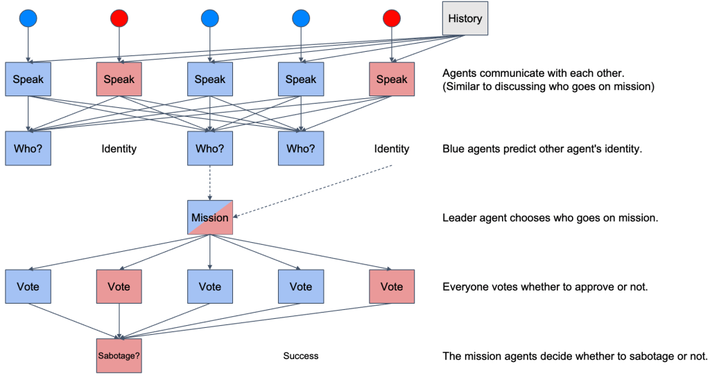
We trained proximal policy optimization (PPO) agents to play the hidden role game The Resistance. Learning whether or not other actors are behaving in your interest, or only pretending to, is a problem widely unstudied in reinforcement learning. We allow the agents to create and develop their own form of communication which allows them to adversarially influence the actions of other agents. We develop several baseline strategies and metrics to evaluate and quantify our training results. A total of 10 models are constructed and used for completing different tasks during the game by two competing teams. We found that the PPO agents can play competitively against our baseline strategies, without training on these baselines. This means the agents not only learn to play against their non-stationary counterparts but learn generic strategies to play against unknown players. Our experimental results show that the agents developed communication in order to identify each other’s roles, resulting in an increase in their win rates. Therefore, we’ve shown that emergent communication is helpful for cooperative and adversarial multi-agent reinforcement learning when there are partially observable states.
The approach for using surface plasmon resonance (SPR) as an optical method for detection of biomolecules with low concentration in real-time has been widely investigated. However, such instruments are highly expensive and bulky, hindering development for portable devices. After discussing with my professor Dr. Lin-Chi Chen about this project, I developed a simple and preliminary platform that can measure the refractive index change of a liquid using SPR.
Figure 1. Prism-based SPR detection
The prism-based SPR system (Fig. 1) is widely used in practical applications, including today’s instruments. Here, A p-polarized light source is refracted into a prism, totally internal reflected (TIR) on another side, and refracted out at another, being received by a light detector. Usually a fluid channel with a special treated surface (e.g. glass with evaporated Au) is placed on the top where the TIR effect happens.
Figure 2. Attenuated total reflection phenomenon (ATR).
When the light beam enters at a certain incidence angle, surface plasmon polaritons can be excited in a resonant manner at the TIR interface. This means there would be attenuated total reflectance (ATR) phenomenon at that angle, and a decrease of light intensity would exist (Fig. 2). This incidence angle is called the SPR angle, and has a linear relationship with the reflection index of the fluid-glass interface.
Hardware Design
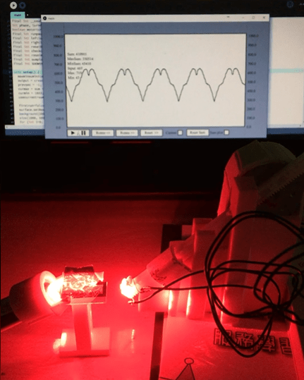
Figure 3. Materials used in this project.
The materials used for constructing this platform are in Fig. 3. As the light emits from the laser, it passes through the convex lens to change its direction, ending up in a slightly diverging beam, entering the prism and hitting the chip surface at different incidence angles (Fig. 4).
Figure 4. Simulation of red light from a laser passing through a convex lens, a prism, and through a microfluidic chip.
The range of incidence angle (Θ) is calculated so that 62.294° < Θ < 72.203°, which at some value within this range there exists the SPR angle of water. Fig. 5 shows a few important specifications for the setup.
Figure 5. Specifications for materials using in this project.
Here’s a clip of the SPR phenomenon appearing at the upper region of the reflected light after an Au-evaporated glass slide is dropped with deionized water.
For detection of light signal, a photoresistor is fixed on a linear gear of the light detector holder. The position of the gear is controlled by a stepper motor fixed on the holder (Fig. 6). The totally internal reflected light will be captured by the moving photoresistor for recording light intensity at a certain position.
Figure 6. Light detection module consisting of a photoresistor, a linear gear, a stepper motor, and a 3D-printed holder.
Program Control and User Interface
Arduino is used for controlling the stepper motor and reading the output of the photoresistor. Prior to reading, the resistances are converted to voltage signals using a simple circuit. For developing a program with visual UI, processing language is used for communicating with Arduino. Fig. 7 shows the program consisting of a signal display panel and several buttons for different functions.
Here’s a demonstration of using the combined UI and hardware platform:
The program will record light intensity, and convert it to a signal with a range between 0 and 1000. In order to calculate the differential signal (the signal with SPR phenomenon minus the signal without SPR phenomenon), the program will average the signal being detected at a certain position within every cycle. By deleting the two averaged signals, this differential signal can be calculated. The differential can indicate the position that the ATR occurred.
Below is another clip for SPR detection using a microfluidic chip, the ATR can be clearly detected by the platform.
The direction of the speed of the linear gear will also have an impact on the signal. In Fig. 8, a smoother SPR curve (average difference of ΔV) is calculated by averaging the data obtained by the clockwise and counter-clockwise direction.
Figure 8. SPR Differential signal of light intensity converted to voltage including clockwise and counter-clockwise directions.
The total cost is a few thousand NTD, which is very low compared with commercial instruments (~1 million NTD). In the future, I hope that this platform can be reinforced for detecting bio-samples in real-time.
The minimization of instruments and relevant devices for data acquisition is a major demand for portable bio-sensing systems. In the following paragraphs, the development of real-time impedance detection systems is detailed, where generations α and β are developed. Generation α serves as the proof-of-concept for the construction of a detection system that can measure impedance from 0.1 to 10000 Hz. Generation β improves several features of generation α, such as the applied frequency range, measured impedance range, detection time, and detection repeatability. In generation β, a website is constructed for controlling the system and acquiring real-time data so that any remote user can have access using smart devices without the need for installing any apps or services. This is particularly useful regarding portability and accessibility, which is highly competitive for integrated biosensors concerning the internet of things (IoT) technologies.
Scheme for Generation α
The general scheme for this generation is depicted in Fig. 1. A function generator is used for producing sine voltage waves across a symmetric electrode system, then a NIDAQ device (USB-6210) is used for collecting voltage signals from the measurement circuit. The signal is processed and sent to a computer for data analysis and plotting.
Figure 1. General scheme for real-time impedimetric detection system (generation α).
Data Analysis using LabVIEW for Generation α
The block diagram and front panel of the LabVIEW data analysis procedure are depicted in Fig. 2. Two signals are acquired by the DAQ device: the input voltage and the amplified current (measured in voltages) of the electrode chip. When the amplification ratio of the current is known, the current can be calculated by dividing the measured voltage with the known ratio. The frequency is calculated using Fourier transform of the signals. The absolute impedance (|Z|) is calculated by dividing the amplitude of the input voltage by the current. The phase angle can be found by calculating the phase difference between the two signals. These two values are plotted on the graph in the front panel and can be saved as comma-separated values (.csv) that can be used for data fitting.
Figure 2. (a) Control panel and (b) block diagram for impedance measurement of Z_GENα using DAQ device and LabVIEW software.
Figure 3. A photo of the whole system of generation α.
The clip below shows real-time impedance measurement using generation α. A microfluidic interdigitated array (IDA) chip (wg/we = 25/100μm, where we is the electrode bandwidth and wg is the gap width) is used. The flow rate is 0.1μL/s and the applied frequency is 100Hz.
A major difference between the detection of phase angle of generation β and that of generation α is that the former always output a sinusoidal wave from a phase angle of 0°, while the latter outputs from an arbitrary angle. By recording the time of the start of detection, the phase angle can be obtained by only measuring the output current wave. For instance, if the peak of a current wave is detected at the start of detection, then it can be deduced that the phase angle is -90° (Fig. 4).
Figure 4. A current wave of phase angle -90°.
In this generation, a miniaturized, portable, real-time, low-cost and remote commandable (website-based) system is developed. The target set for it has a whole list of goals in addition to the main features of a typical impedance analyzer: miniaturization, portable, real-time, low-cost and user-friendly. For the hardware, a Raspberry Pi 3 b+ model, an impedance measurement circuit, and a microelectrode sensor chip are integrated. The scheme of generation β is illustrated in Fig. 5.
Figure 5. General scheme for real-time impedimetric detection system (generation β).
Impedance Measurement Circuit Design
For generation β, several IC chips are integrated on a universal PCB board for achieving the functions of the function generator and the DAQ device in generation α. The AD9833 waveform generator is used for the production of sinusoidal voltage waves. TL074op-amps are used for transformation of electric signals. The fast precision op-amp OP42 is used for amplification of the small signal current running through the sensor chip. A voltage stabilizer module made from UA741 op-amp is used for providing stable voltage signal. The analog-to-digital converterAD7822 is used for signal acquisition, and sending digital signals to Raspberry Pi (Fig. 6).
Figure 6. Circuit schematic for generation β.
Data Processing
The raw signal obtained by the ADC is an 8-bit resolution data ranging from 0 to 255 at a rate of 1MS/s (mega samples per second). Due to the relatively fast sampling speed by Raspberry Pi and some imperfections within the circuitry, there may appear to be some defects or noisy signal in the acquired data. Thus, a strategy for data processing before the calculation of |Z| and phase of the measured system is designed. The general concept is depicted in Fig. 7 for a raw signal with a linearly transformed value between 0 and 1.
Figure 7. Strategy for impedance range detection and data processing for generation β.
First, leading and ending consecutive zeros are trimmed, and the data is shifted to a start of a non-zero value. Second, values outside n standard deviations from the average of m data points are removed where n and m are arbitrarily defined constants for a specific sampling frequency. Third, the removed values are linearly bridged between non-removed values to form continuous data points. Fourth, smoothing is performed by averaging k data points to form a new value. |Z| is found by calculating the standard deviation of the overall data which equals the zero-mean root-mean square (RMS) of the signal and is proportional to the amplitude with a relationship of . The phase is obtained by first calculating the average of the remainder of the time (μs) of a data point, which is larger than or equals the mean and its previous data point is smaller than the mean, divided by the number of data points within a repeating sine wave cycle, then linearly transforming it to a value between 0 and 360 degrees.
Website Server
For portable devices dedicated to point-of-care applications, a miniaturized device must be set up that contains user-friendly interfaces and well-designed data display graphics. A smart phone might come in handy when it comes to the such integration. Applications using smart phone for electrochemical on-chip detection of biomarkers are presented and published every year. For the above reasons, a website platform for the user interface of generation β is set as a target for its improvement compared with generation α, which can be accessed using local networking on either a personal computer, a smart phone, a pad … etc. The overall structure is shown in Fig. 8.
Figure 8. Structure of the web server of generation β.
Results for Generation β
The photograph of generation β is shown in Fig. 9. The dimension is 22(L)×10(W)×6(H) cm3, which makes it a portable system. The Raspberry Pi controls the circuitry by sending voltage signals towards the IC chips. The sinusoidal current passes through the sensor chip, gets amplified, then is sampled by the ADC. The transformed digital values are read by the Raspberry Pi and being processed. At last, impedance values are plotted on the website.
Figure 9. Photograph of generation β.
The content below is a clip for demonstration of using the website interface of generation β. The website shows |Z| vs f, phase vs f, Im(Z) vs Re(Z), Re(Z) vs f and –Im(Z) vs f at the same time. The collected data can be saved to a CSV file for further analysis.
A mobile power supply can be simultaneously used as the power supply for the circuitry and Raspberry Pi (Fig. 10), and smartphone-controlled impedance detection can also be achieved (also shown in clip below).
Figure 10. Generation β powered by a power bank.
Microfluidic Impedimetric Detection using Interdigitated Au Electrode Chip
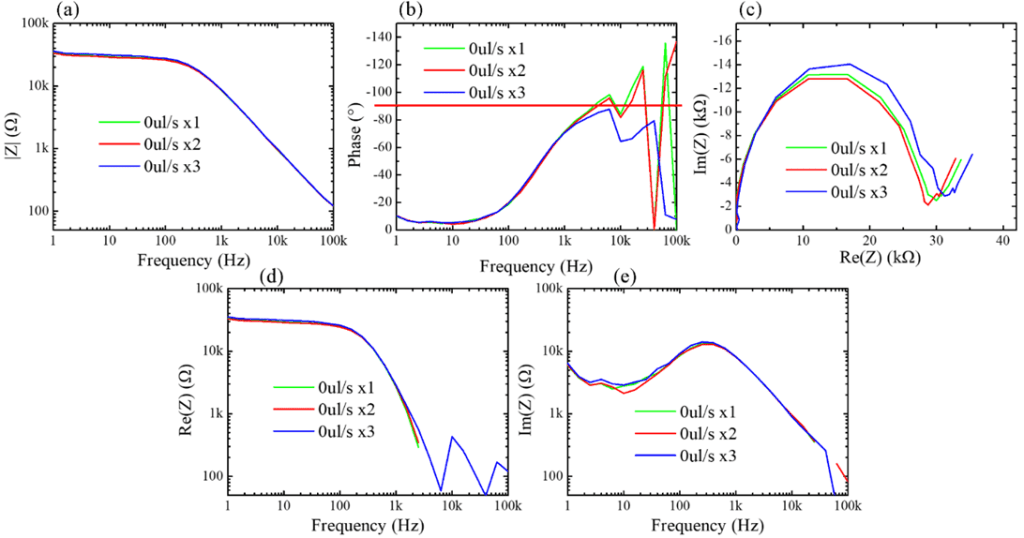
The repeatability of electrochemical impedance spectroscopy (EIS) detection in a microfluidic interdigitated array (IDA) chip system is tested using generation β as the measuring system. In Fig. 11, it can be seen that a fairly stable measurement of |Z| can be achieved within a frequency range of 1 ~ 105Hz, and an absolute impedance range of about 0.1 ~ 30kΩ can be detected. However, at high frequencies, the phase angle does not have a reasonable and repeatable value. This reason is due to the larger noise of sampling values at high frequencies. A red line is drawn at 90° on the phase vs f plot. Normally, phase angles wouldn’t exceed this value because that would give rise to a negative Re(Z), and does not correspond to any familiar electrochemical mechanism. Such sampling errors and data processing are needed to be improved.
Figure 11. (a) |Z| vs f, (b) phase vs f, (c) Im(Z) vs Re(Z), (d) Re(Z) vs f and (e) Im(Z) vs f for single EIS detection of IDA chip at 0μL/s flow speed using generation β. The channel width is 0.5mm. Vamp = 50mV. Running buffer: 5mM Fe(CN)63-/4-in PBS.
It is already well-known that in 2016, the computer program AlphaGo became the first Go AI to beat a world champion Go player in a five-game match. AlphaGo utilizes a combination of reinforcement learning and Monte Carlo tree search algorithm, enabling it to play against itself and for self-training. This no doubt inspired numerous people around the world, including me. After constructing the automated forex trading system, I decided to implement reinforcement learning for the trading model and acquire real-time self-adaptive ability to the forex environment.
Environment Setup
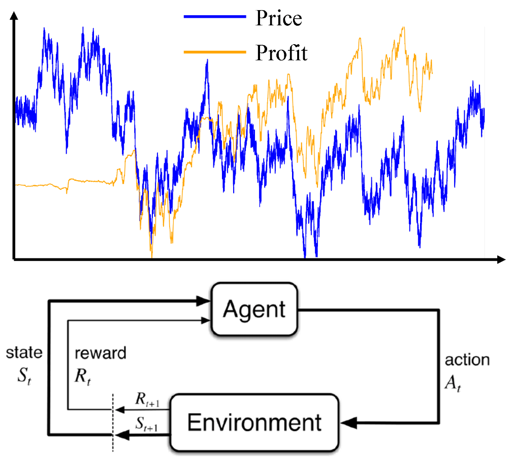
The model runs on a Windows 10 OS (i9-9900K CPU) with DDR4 2666MHz 16G RAM and NVIDIA GeForce RTX 2060 GPU. Tensorflow is used for constructing the artificial neural network (ANN), and a multilayer perceptron (MLP) is used. The code is modified from the Frozen-Lake example of reinforcement learning using Q-Networks. The model training process follows the Q-learning algorithm (off-policy TD control), which is illustrated in Fig. 1.
Figure 1. Algorithm for Q-learning and the agent-environment interaction in a Markov decision process (MDP) [1].
For each step, the agent first observes the current state, feeds the state values into the MLP and outputs an action that is estimated to attain the highest reward, performs that action on the environment, and fetches the true reward for correcting its parameters. The agent follows the epsilon-greedy policy (ε = 0.1) for striking a balance between exploration and exploitation.
State, Action and Reward
For the 1st generation, price values at certain time points and technical indicators are used for constructing the states. The technical indicators used are the exponential moving average (EMA) and Bollinger bands (N=20, k=2), and time frames of 1, 5 and 15min are used with the last 10 time points being recorded. A total number of 36 inputs are connected to the MLP.
There are three action values for the agent: buy, sell and do nothing. The action being taken by the agent is determined by the corresponding three outputs of the MLP, where sigmoid activation functions are used for mapping the outputs to a value range of 0 ~ 1, representing the probability of the agent taking that action.
For the reward function, the difference between the trade price (the price when a buy/sell action is taken) and the averaged future price is considered. If a buy action is taken, then the reward function is calculated by subtracting the averaged future price with the trade price; if a sell action is taken then the reward is calculated the other way around. For “do nothing” actions, the reward is 0. A spread is subtracted from the reward for buy/sell actions to obtain the final reward. This prevents the agent to perform actions that result in insignificant profit, which would likely lead to a loss for real trades (Fig. 2).
Figure 2. Reward calculation method for buy/sell actions.
Noisy Sine Function Test
For preliminary verification of effectiveness for the training model and methods, a noisy sine wave is generated with Brownian motion of offset and distortion in frequency. This means at a certain time point (min), the price is determined by the following equation:
where Pbias is an offset value with Brownian motion, Pamp is the price vibration amplitude, T is the period with fluctuating values, and Pnoise is the noise of the price with randomly generated values. (Note that the “price” mentioned here is defined as the exchange rate between two currencies)
Fig. 3 shows a randomly generated price vs time sequence within a range of 50,000 minutes with an initial values Pbias = 1.0, T = 120 min, Pamp = 0.005, and Pnoise amplitude = 0.001. Generally, the price seems to fluctuate randomly with no obvious highs or lows. However, if it is viewed close-up, waves with clear highs and lows can be observed (Fig. 4).
Figure 3. Price vs time of the noisy sine wave from 0 to 50,000 min.
Figure 4. Price vs time of the noisy sine wave from 20000 to 20600 min.
The whole time period is 1,000,000 min (approximately 700 days, or 2 years). Initially, a random time period is set for the environment. Every time the agent takes an action, there is a certain chance (= 1%) that the time will jump to another random point within the whole period. Otherwise, the time will move on to a random point which is around 1 ~ 2 day(s) in the future. This setting is expected to correspond to real conditions, where a profitable strategy can have stable earnings and can also adapt quickly to rapid changing environments.
Fig. 5 plots the cumulative profit for trading using the noisy sine wave signal for 50,000 steps. Although it took approximately 25,000 steps to make the model get “on track”, I recognize this result as an important start for implementing real data.
Figure 5. Cumulative profit from trading using a noisy sine wave signal.
Fundamental Analysis for Economic Events
Fundamental analysis is a tricky part in forex trading, since economic events not only correlate with each other, but also might have opposite effects on the price at different conditions. In this project, I extracted the events that are considered significant, and contain previous, forecast and actual values for analysis. Data from 14 countries of the past 10 years are downloaded and columns with incomplete values are abandoned, making a complete table of economic events.
Because different events have different impacts on forex, the price change after the occurrence of an event is monitored, and a correlation between each event and the seven major pairs (commodity pairs). Table 1 displays a portion of the correlation table for different economic events. The values are positive, which indicates the significance of an event on the currency pair. Here, a pair is denoted by the currency other than the USD (e.g. USD/JPY is denoted as JPY).
Table 1. Correlation table between 14 events and 5 currency pairs. Here, a pair is abbreviated as the currency other than the USD.
Country
Economic Event (Index)
AUD
CAD
EUR
GBP
JPY
AUD
Commodity Prices
0.00313
0.00268
0.00266
0.00339
0.00278
AUD
MI Inflation Expectations
0.00338
0.00168
0.00217
0.00200
0.00266
AUD
RBA Interest Rate Decision
0.00428
0.00262
0.00258
0.00298
0.00225
EUR
Manufacturing PMI
0.00331
0.00284
0.00263
0.00298
0.00278
EUR
Italian CPI
0.00315
0.00319
0.00295
0.00316
0.00255
EUR
Services PMI
0.00341
0.00290
0.00293
0.00295
0.00284
EUR
CPI
0.00304
0.00294
0.00262
0.00317
0.00241
EUR
German Unemployment Rate
0.00315
0.00315
0.00273
0.00313
0.00246
EUR
ECB President Trichet Speaks
0.00344
0.00248
0.00341
0.00302
0.00268
EUR
German Unemployment Change
0.00313
0.00313
0.00268
0.00307
0.00243
EUR
German Trade Balance
0.00306
0.00255
0.00300
0.00284
0.00268
EUR
German Factory Orders
0.00292
0.00265
0.00312
0.00280
0.00275
EUR
German Retail Sales
0.00304
0.00304
0.00353
0.00310
0.00275
EUR
French Trade Balance
0.00312
0.00312
0.00296
0.00301
0.00299
A total of 983 events are analyzed. However, due to the fact that a large portion of events have little influence on the price, only 125 events that have a relatively significant impact are selected as the inputs of the MLP.
Real Data Implementation Results
Per-minute exchange rate data of the seven currency pair is downloaded from histdata.com. A period from 2010 to 2019 is extracted, and blank values are filled by interpolation. This gives us a total of approximately 23 million records of price data (note that weekends have no forex data records), and is deemed sufficient for model training. The data is integrated into a table, and technical indices are calculated using ta, a technical analysis library for Python built on Pandas and Numpy.
Figure 6. EUR/USD exchange rate from 2010 to 2019.
Summing the inputs from technical analysis, fundamental analysis, and pure price data, a total of 1049 inputs are fed into the MLP. Within the hidden layers, ReLU activation is used, and a sigmoid activation function is used for the output layer. The output has a shape of 7×3, which represents the probability of the seven currency pairs and the three actions (buy, sell, do nothing).
Fig. 7 shows the accumulative profit from 2,000,000 steps in a single episode and its win rate (percentage of profitable trades within a moving average). An increasing spread value from 0.00001 to 0.00004 is applied, which the spread value starts from 0.00001 and increases by 0.00001 every 50,000 step. It can be seen that overall, the accumulative profit rises steadily. However, the win rate usually falls below the 50% line. How could a profitable trading strategy be possible? This is due to the fact that the average profit of a winning trade (=0.003736) is larger than the average loss of a losing trade (=0.003581). Thus, the overall result is a profitable trading strategy.
Figure 7. Accumulative profit and win rate from the training procedure of 2,000,000 steps.
Conclusion
In conclusion, a trading model for profitable forex trading is developed using reinforcement learning. The model can automatically adapt to dynamic environments to maximize its profits. Although for real conditions that have a larger spread, the model hasn’t achieved a stable and profitable result, the potential for optimizing is promising. In the future, I am planning to integrate this trading model with the automated forex trading system that I have made, and become a competitive player in this fascinating game of forex.
I have always wanted to automate the cumbersome experimental operation process. For biochemical experiments, often a whole day in web lab is spent in order just to acquire one single set of data. Having the hands-on experience of developing hardware and software integrated systems for several projects (e.g. Surface Plasmon Resonance Platform, Real-time Impedance Detection Systems), I initiated this project for constructing a microfluidic controlling platform that can automatically manipulate liquid-based solutions of little volume, and also assist real-time detection experiments.
Platform Structure
The platform is constructed by four sections: A Raspberry Pi, an actuator module that consists of an Arduino and two H-bridge circuits, a fluid controlling system made up of a syringe pump/syringe device, and the microfluidic platform (Fig. 1).
Figure 1. System architecture of the automated microfluidic controlling platform.
Here, the Raspberry Pi serves as the main processing unit, which an Apache web server is constructed on, and is used to communicate with a remote user by website. The front-end of the website is designed using HTML, Javascript and CSS, and the back-end is designed using PHP. Javascript and PHP communicate using jQuery, and the PHP code is written for controlling peripheral devices.
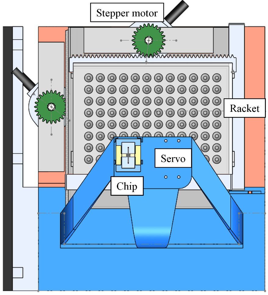
For x/y position control, the Raspberry Pi sends data through type-B USB to the Arduino, which afterwards commands the H-bridge circuits, then control the x/y stepper motors on the microfluidic platform for moving the position of the racket. The servo motor is used to control the high/low position of the tube it holds, where the high (low) position means the tube isn’t (is) inserted into the microtube (Fig. 2).
Figure 2. The microfluidic platform and surrounding modules.
For fluid control, the Raspberry Pi sends an infuse/withdraw signal to the syringe pump using another type-B USB, which subsequently pushes/pulls the syringe on it. A simple flow for moving liquid from microtube A to microtube B is:
1. Confirm that the tube (for fluid conveyance) position is high. If not, then move it up by servo motor. 2. Move to microtube A by stepper motor. 3. Change tube position to low by servo motor. 4. Withdraw liquid by syringe pump. 5. Change tube position to high by servo motor. 6. Move to microtube B by stepper motor. 7. Change tube position to low by servo motor. 8. Infuse liquid by syring pump.
Figure 3. Photograph of the automated microfluidic controlling platform.
The circuitry for this platform is relatively easy compared with other projects (e.g. Aroma Alarm Clock), and is consisted simply with wires and resistors. Except the motors and the racket with microtubes, all the other components of the for microfluidic platform are fabricated using 3D printing. 3D-printed gears are fixed with the stepper motors. Precise control of racket position (~ 0.2mm) is realized by combining the gears with a 3D-printed linear gear that fits on the racket and another linear gear of a subsidiary platform which the racket sits on. Below is a clip demonstrating how the 3D-printed components, the stepper motors, the racket with microtubes, and a microfluidic electrode chip are integrated together, along with x/y position control of the racket.
Software Development
The program structure written inside Raspberry Pi is quite similar to the program structure in another project “Real-time Impedance Detection Systems”. The difference for this project is that PHP is used to directly communicate with peripheral devices (Fig. 1).
Fig. 4 displays the website-based user interface for controlling this platform. The UI is divided in four sections: procedure window, buttons field, racket window, and status window. Briefly, the user can save/load settings from the connected Arduino, add/delete a control command, start/pause/stop the current procedure, download the control procedure to a text file, and append a command after another one.
Figure 4. Website user interface of the platform.
Fig. 5 shows the settings menu. Here, the user needs to find the device url for Arduino and the syringe pump beforehand and insert them. Several controlling preferences, such as motor operation delay time, steps for the stepper motor to move per cell (microtube), precise high/low position of the servo motor, current cell of the racket … etc. can be set.
Figure 5. Settings menu of the UI.
Fig. 6 shows the add command menu. The user can either move the stepper motor to a target cell (microtube), infuse/withdraw fluid at a self-defined rate and target volume, move servo high/low position, or perform a time delay.
Figure 6. The add command menu of the UI.
Concentration Gradient Generation
An automated concentration gradient generation process is written, and is carried out by the automated platform. Here is a clip for demonstration (speed = 10x):
Real-time Impedimetric Detection
The tube doesn’t have to directly connect to a syringe. A detection chip can be inserted between for real-time detection of different solutions (similar to the method illustrated in Fig. 1 of another project Surface Plasmon Resonance Platform). A microfluidic interdigitated electrode chip using microfabrication technique is previously developed (which is a part of my research), and is used for detection of electrochemical impedimetric properties of the fluid. Here, potassium ferricyanide (K3Fe(CN)6) and potassium ferrocyanide (K4Fe(CN)6) are serial diluted using the platform, and real-time impedance detection is carried out using an electrochemical analyzer (CHI614b, CH Instruments) and the microfluidic chip.
Fig. 7 shows the detection result. It can be seen that the solution switching time is relatively fast and stable, and the detection time is consistent, which demonstrates the advantages of this automated platform.
Figure 7. Real-time impedimetric detection plot for different diluted concentrations of K3Fe(CN)6/K4Fe(CN)6.
Summary
In summary, a website-controlled automatic microfluidic controlling platform is designed and fabricated for real-time microfluidic sensing and other applications. Solution manipulation using this platform is stable, repeatable, and time-saving compared with manual operation.
As an old saying goes, “An hour in the morning is worth two in the evening”. What we encounter and conceive during this period is largely intertwined with our whole day. However, what is the most important thing that we encounter in the morning? It is about waking up. Nowadays, we wake up by the noisy, buzzing sound of an alarm. How would it be like if we could wake up by a scent, a fragrance, wiping away the unsatisfactory memories of the past? What can be changed to fulfill a better awakening?
An aroma alarm clock should fill in the answer. When I was a junior, I enrolled in a program called “NTU Creativity and Entrepreneurship Program” (NTUCEP). In this program, students with similar ideas form groups and learn about entrepreneurship by practice. After a couple days of brainstorming, our group came up with the concept about developing an alarm clock that can wake people up using scent packs. Apart from being awakened by a loud ringing sound of an alarm, fragrances (as we had proposed) have a milder, progressive effect for waking people up. We named our product “Sensio”, a Latin noun of the meaning “thought”.
Market Survey
In order to verify the market demand of this proposal, we devised a questionnaire for investigating the views and habits of people about waking up, which 1320 valid responses were collected. A score of 0 ~ 7 is used to quantify the “discomfort level” for waking up, in which a level of 0 ~ 3 is regarded as painless, and 4 ~ 7 as painful. Fig. 1 shows the discomfort level distribution of all the samples, and Fig. 2 shows the distributions by occupation. It can be seen that regardless of identity, the majority of people feel painful when waking up (students: 71%, office worker: 62%, other: 51%, overall: 68%). Moreover, we analyzed their habits of lying in bed after awakening. Fig. 3 shows the proportion and durations for lying in bed. Accordingly, over 44% of people lie in bed for over 15 minutes, and the average duration is 15.07 minutes. Theoretically, this means if a product could help lower one’s discomfort level of waking up, and reduce the duration of lying in bed after awakening, he could approximately increase 3.8 days/year of effective time. Not only having a favorable morning, but also enhancing his work efficiency.
Figure 1. Discomfort level distribution of waking up.
Figure 2. Number of people vs discomfort level by occupation.
Figure 3. Duration of lying in bed after awakening.
From the above analysis, we became confident about the large market demand for a better quality of getting up. For me, being the leading engineer role in our group of six meant turning ideas into reality. This had been a difficult period but a time of inspiration and excitement. I put into practice what I had learned within the past few years for developing a system, a hardware that can really be used as a product.
Sensio v0.1
I developed two preliminary versions of the hardware, with the 1st version using Arduino as the CPU (Sensio v0.1) (Fig. 4). In this version, an Arduino chip, a time clock module (DS1302), a shift register (74HC595N), relays, button switches, LED displays, a buzzer, a fan and a potentiometer are used for the alarm clock (Fig. 5). 10 different themes are written inside the system and a few simple features are integrated within (Fig. 6 details every mode of the alarm clock and the corresponding function of the buttons). This version serves as the proof-of-concept version for making an aroma alarm clock. Although being simple and somewhat rough, it demonstrated to my team and our professors a solid proof and feasibility of our objective.
Figure 6. Alarm modes and button function for Sensio v0.1.
During this period, we earned 40,000NTD in a fundraising event in our program, and won the Best Potential Award in the 14th NTU innovation competition. Fig. 7 shows the poster we had used in the competition. During that period, we had great enthusiasm and motivation, and dreamed that one day our product would become on-sale and we could establish a real listed company of our own. We entered the NTU garage, which is an incubator for startups that are closely linked to NTU.
Figure 7. Poster of product Sensio for the NTU innovation competition.
Sensio v0.2
The second version Sensio v0.2 was created during my second semester as a junior. This time, an IC chip (ATMEGA328P) is used as the CPU rather than Arduino in order to lower the cost of the system and decrease its volume. Moreover, a PCB layout for fixing electronic parts on a solid panel is used. Fig. 8 illustrates the structural model of Sensio v0.2, Fig. 9 shows a photograph of the integrated electric components and its corresponding PCB layout schematic, and Fig. 10 shows photographs of the laser-cut 3D outer case.
Figure 9. Electronic component-integrated PCB board of Sensio v0.2 and its corresponding layout schematic.
Figure 10. Outer case (blue) and scent pack holder (orange) of Sensio v0.2.
We were thrilled after these accomplishments, since never had a team of the same period achieved such a high level of completeness, especially when concerning the integrity of hardware and software. These remarkable things happen so quickly, so fleeting for us to catch up with. The truth is, we are still so far from success, since we were still students back then. Reality pulled us back, and we started asked ourselves: are we ready to give up some things and dedicate ourselves to entrepreneurship? Our dream product, the aroma alarm clock, had once seemed so close, yet had never seemed so far.
Although in the end, the functional aroma alarm clock wasn’t successfully made, what I’ve learned during this event is unprecedented compared with my past experience, not only techniques for hardware and software development, but also important philosophies for entrepreneurship. This project inspired me to a great extent, and enabled me for creating future hardware-related projects (e.g. Automated Microfluidic Controlling Platform, Real-time Impedance Detection Systems, Surface Plasmon Resonance Platform) in my own field of research.
I started to use a technique called electrochemical impedance spectroscopy (EIS) for biosensing since my undergraduate research. For analyzing EIS data, an equivalent circuit must be constructed for modeling the reaction mechanism. Physical parameters can be extracted by fitting the data using the model. However, for most software, the circuit elements being provided and their corresponding combined circuit couldn’t necessarily meet my needs for finding the physical parameters in a symmetric electrode system. Therefore, I developed a circuit fitting program for customized analysis of impedance data. The fitting and impedance calculation program are used in a first-author journal paper of mine. In the following paragraphs, the development of the fitting program, another program that assists data visualization, and a program for calculating the diffusion impedance of interdigitated array (IDA) electrodes are detailed.
Figure 1. (a) The Nyquist plot for visualizing impedance values, and (b) an equivalent circuit with several circuit elements for modeling electrode surface reactions.
Electrochemical Impedance Circuit Fitting Program
The algorithm for finding all the element parameters in a given circuit is by implementing the Levenberg-Marquardtnon-linear fitting method. This is a general and popular method for solving the minimum value of function E(x), where
$$E(x)={1 \over 2} \sum_{i=1}^m [f_i(x)]^2 $$
For impedance data fitting, a complex non-linear least square process (CNLS) is implemented, and the above equation can be specialized as
where S is the weighted sum of squares of error, Nf is the number of frequencies within an experiment, Zi is the impedance of the i–th frequency, and wi,Re and wi,Im are the statistical weights for the real and imaginary parts of the impedance of the i–th frequency. The subscript exp indicates experimental value and the subscript cal indicates the calculated value while fitting.
For any kind of circuit, Zi,cal can be calculated by the set of element parameters and the frequency (e.g. R for a resistor, C and f for a capacitor), then S can be calculated using its defined equation. By minimizing S, the fitted element parameters can be modified so that the result impedance (Zi,cal) can be as close as possible to the experimental value (Zi,exp). Fig. 2 shows an example for a non-linear curve fitting process.
A program written in C language is designed using the open-source numerical analysis library ALGLIB® to implement numerical integrations and calculations. ALGLIB is also used for non-linear least squares fitting of EIS data using Levenberg-Marquardt method. Several circuit elements for EIS data fitting are available in this program, which are shown in Table 1. Detailed methods for calculating the IDA diffusion element is shown in my first-author paper.
Table 1. Available circuit elements in the fitting program.
A circuit description code is defined to express equivalent circuits. Elements, including whole blocks inside parentheses, are either in series or parallel with each other. Those inside an odd number of pair of parentheses are in parallel with each other, and those inside an even number of pair of parentheses are in series. Fig. 3 shows a circuit equivalent to the description code of “R(RC)(R(RC))”.
Figure 3. Circuit description code and its corresponding circuit. Equivalent parts are marked by identical colored blocks.
Figure 4. Snapshot of the equivalent circuit fitting program.
It is reasonable that an element in a circuit contributes to the impedance change to a certain degree. For instance, a resistor has an influence on the real part of impedance, and a capacitor affects its imaginary part. However, when the circuit consists of elements with serial or parallel combinations, it can be quite difficult to imagine how the shape of impedance data would change according to each element.
Therefore, I wrote a program for plotting impedance data in real-time using Processing language. After entering the circuit description code into the program, a Nyquist plot, total impedance Bode plot, and phase angle bode plot is generated. The user can use horizontal bars to control the value of a specific element. By changing its value, the impedance would be calculated immediately, and the plot would be drawn out in real-time.
Figure 5. User interface for the real-time impedance plotting program.
Here’s a clip for demonstrating the real-time impedance plotting program.
The IDA diffusion element is a novel element for parameterizing the diffusion impedance of an IDA electrode using its shape factor (we/w), magnitude of the admittance (Y0), and the dimensionless frequency (w2ω/D). However, complex functions are required for calculating its value, such as the Bessel function, the complete elliptic integral of the second kind, and definite integrals.
Due to calculation difficulties, a program is written for calculating the IDA diffusion impedance. The program consists of two files “settings.txt” and “IDA_diff_Z.exe”. “settings.txt” is of the format below:
These contain all the 12 parameters for the usage of this program. A detailed description is listed in order below:
If [output to txt file] is 0, then calculated impedances will be shown directly on screen. If it is 1, then the values will be saved to the file “Z_diffusion_IDA.txt”.
The maximum frequency for impedance calculation can be set after [max freq (Hz)].
The minimum frequency for impedance calculation can be set after [min freq (Hz)].
The number of frequency points within a decade can be set (e.g. If [points per decade] is set to 5, then frequencies calculated between 101 and 100Hz will be 101, 100.8, 100.6, 100.4, 100.2 and 100Hz.)
we can be set after [electrode bandwidth we (um)].
wg can be set after [gap width wg (um)].
l can be set after [electrode length l (mm)].
N can be set after [number of bands N].
D can be set after [diffusion coefficient D (m^2/s)].
C* can be set after [bulk concentration C* (mM)].
n can be set after [number of electrons n].
T can be set after [temperature T (K)].
After setting the 12 parameters, put “settings.txt” and “IDA_diff_Z.exe” in the same directory and open “IDA_diff_Z.exe”. Impedances will be automatically calculated and printed in the defined format (Fig. 6). ※The program can only be run in a Windows 64-bit environment.
Figure 6. An example output of the IDA diffusion impedance calculation program.