Lyto Different Color is a color differentiation game on Facebook. Each level, there are NxN circles on a board, with one circle having a color slightly different from all the others. The player must find the circle with different color and click on it in order to go to the next level. During the early stage of the game, the difference between the color of the unique circle and the color of the other circles gets smaller, and N gets larger, making it become more difficult. For most people, level 50 is considered a high score, and it is almost impossible for a normal human to reach level 100.
I simply wanted to break this limit, so I wrote a Python script for continuously taking a snapshot of the section of the game screen, find the circles, reading their color, and pressing on the circle with unique color. It is comparatively easy for the AI to recognize the differences, since it reads the colors as an RGB value, where any difference in the values represents a difference in color.
Python Imaging Library (PIL) is used for capturing the game screen, which approximate takes a screenshot every 0.7 seconds. Afterwards, the boundary of the circles is found by finding pixels that have a different color compared with the plain background color. Then, N is found by counting continuous blocks of identical colors from a 1D diagonal slice of array from the top-left to bottom-right corner of the boundary. By finding these values, the center of every circle can be located, which the program retrieves the colors from and compare them. At last, the circle with unique color is found, and the program sends a signal to the mouse for pressing on the target position. Fig. 1 illustrates a graphical description of the program algorithm.
Figure 1. Graphical description of the algorithm for Lyto Different Color AI.
Here’s a clip of the program playing the game (2x speed):
My research as a graduate student focuses on biosensing applications using electrochemical impedimetric methods. Unlike mechatronic systems, these applications consider a dynamic environment at such a microscale, it is quite hard to perceive what is really going on when we merely recognize the change of physical property. I usually ask myself: What is the underlying mechanism? Tucked away from the limit of horizon of the human eye, we often see nothing happening when doing these experiments.
The result of task 1 supports the hypotheses of task 2 and 3.
Physical Environment Setting
The simulation environment is set as the interior of a microfluidic channel with gold microelectrodes. See the film below for visualization.
The chip is fabricated using soft lithography and photolithography. The microfluidic channel has a width of 1mm and a height of 100μm at the center. The gold microelectrodes form a pair for square pads (300×300μm) at the center of the channel (Fig. 1).
Figure 1. Microfabrication process, dimensions, and microscopic view of the microfluidic electrode chip used in this project.
Velocity Field Simulation Inside Microfluidic Channel
The objective of this task is to simulate the fluid velocity field inside the channel on a sliced plane. Due to the fact that 3D simulation is time-consuming, if a 3D environment can be reduced to a 2D environment, then a large amount of time can be saved. By performing this task, it can be seen if dimension reduction modeling of task 2 and 3 are feasible.
Considering the physical nature of the microfluidic channel, a laminar flow model is implemented along with the Navier-Stokes equation:
, which means a balance between inertia (\(\rho(\textbf{u}\cdot\nabla)\textbf{u}\)), pressure (\(-pI\)), viscous (\(\mu(\nabla \textbf{u}+(\nabla \textbf{u})^T)\)) and external (\(F\)) forces. A stationary study is implemented (\(\rho \nabla \cdot \textbf{u}=0\)), and water is set as the fluid.
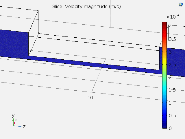
Fig. 2 shows the 3D velocity field inside the channel. A bigger arrow indicates a larger velocity magnitude. The reason that the velocity is faster at the center is because of the lower channel height.
Figure 2. 3D velocity field inside microfluidic channel.
Fig. 3 shows animated 2D velocity fields of sliced planes inside the channel. Due to laminar flow, velocities near the boundary get close to zero. However, the steady-state velocity reaches a constant value away from the boundary.
Figure 3. 2D velocity fields for xy and zy sliced planes.
A top view of the velocity field and the velocity at different x positions are shown in Fig. 4. It can be concluded that at the center of the channel where the microelectrodes lie, the fluid velocity stays constant, and subsequent tasks can be carried out using 2D models.
Figure 4. Top-view and x position-dependent velocity magnitude of fluid.
Real-time Molecule Immobilization on Gold Surface.
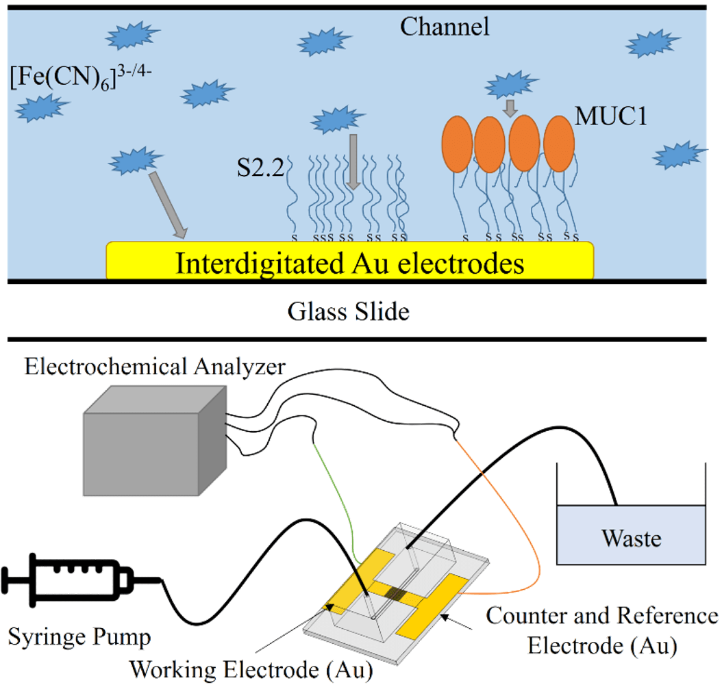
For microfluidic electrochemical biosensors, it is quite common that immobilization of sensing elements takes place at the center of the channel on electrode surfaces (e.g. Au). In this task, molecules are simulated to flow past the channel, and be immobilized on the electrode pad at the bottom center. A slice on the zy plane is used as the modeling geometry of this task (Fig. 5).
Figure 5. Modeling geometry used in task 2. A sliced area of the microfluidic channel with pad electrode at the bottom center is used.
Here, the molecules convect and diffuse near the surface, the rate of immobilization is determined by several factors including the inlet concentration (c0), diffusion coefficient (D), maximum surface molecule density (Γs). The convection-diffusion equation and transport-adsorption equation are used along with time-dependent study:
$${{\partial c} \over {\partial t}} + \nabla \cdot (-D\nabla c) + \textbf{u} \cdot \nabla c = R$$
For the transport-adsorption equation, it is assumed that the change of surface concentration plus the rate of surface diffusion equals the rate of Langmuir adsorption isotherm.
Fig. 6 shows the time-dependent surface concentration (cs) change when c0 = 1μM, and Fig. 7 shows the binding curve (probe density vs time) for different values of c0.
Figure 6. Time-dependent surface concentration (cs) change. t = 0~18hr.
Figure 7. Probe surface density (molecules/cm2) vs time (hr).
At concentrations above 0.1μM, the probe density almost saturates to a value of 9.6×10¹² molecules/cm2 before immobilizing for 10 hours. The result highly resembles a typical binding curve, suggesting the possibility for computer simulating assisted optimization of in vitro parameters, which is really helpful for understanding underlying mechanisms for the system.
EIS is a rapid and label-free method for detection of bio-molecules, and is widely implemented on a variety of biosensors. In this task, I simulated EIS diagrams by changing the values of the heterogeneous rate constant (k0) and the double layer capacitance (Cdl). Both Cdl and k0 are affected by the immobilized surface molecule density on an electrode surface, and are important physical properties when analyzing EIS data. A slice on the xy plane is used as the modeling geometry of this task (Fig. 8).
Figure 8. Geometry being simulated for task 3. A 2D plane is sliced in the xy direction.
Here, a sinusoidal voltage wave is applied between the two electrodes (amplitude ≅ 5mV), and Bode plots and Nyquist plots can be drawn according to the measured impedance. According to the surface redox reaction, an equivalent circuit can be constructed. The equivalent circuit for this task is shown in Fig. 9.
Figure 9. Equivalent circuit used in my research and task 3.
EIS plots are simulated for different values of k0 and Cdl (Fig. 10).
Figure 10. Bode and Nyquist plots for the simulated EIS data. k0 has a range from 0.001 to 0.1 (cm/s), and Cdl has a range from 0.01 to 100 (uF/cm2).
By undergoing this simulation project, I furthermore understood some fundamental interactions between the physical properties and outcome of my research to a new depth, and developed new concepts about how to improve it.
This is an end semester project that I have done with my groupmates in college. In this study, we proposed a model to predict a startup company’s future condition using a deep multilayer perceptron (MLP) and decision tree. I mainly played the role for data quantification and literature review of this study. In our study, we built a prediction analysis model for startup companies. Furthermore, we identified what the key factors are and what influences will it have on the results. Our main hypothesis is that money, people and active days are the key factors. We built the prediction model from CrunchBase, which is the largest public database with relevant profiles about companies.
Data Quantification
For the data obtained, there are 4 groups of data that are quantified: country state, employee range, roles and countries. Regarding the states group (which only exists in USA and Canada), we think that different states have different impacts on the survival rate of a startup. A lookup table for scoring of states is defined [1][2][3]. The original data for employee quantities are a range between two numbers (e.g. 101-250). These are transformed into the average of the upper and lower bound. Employees of 10000+ are defined to be 15000. For the roles group, the data “company” is arbitrarily defined as 0.1 and “company, investor” is defined as 0.9. This is because we regard a company as wealthier and influential when it also plays a role of an investor, compared with only being a company. The other roles are transformed to 0.5. The impact of country on startup environment is also studied [4] and scores from 0.329 to 0.947 are given to countries that have above 300 startup companies in record.
Table 1. Company status and scores of 23 countries.
The ANN runs on a Windows 10 OS (i7-8700k CPU) with DDR4 2666MHz 16G RAM and Nvidia GTX 1070 Ti GPU. Keras is used to construct the network, and three networks of multilayer perceptron (MLP) with different number of layers are designed for comparison. There are 4 outputs of the network, indicating the probabilities of the final status which are: (1) Closed, (2) Operating, (3) Acquired and (4) IPO.
Figure 1. MLP Structure of the 3 neural networks.
The three networks have respectively 2, 4 and 6 hidden layers, with each network all starting with a 1024-neuron hidden layer and ending with a 32-neuron hidden layer (Fig. 1). Table 2 shows the training results.
Table 2. Mean square error (MSE) and categorical cross-entropy loss for the 3 networks.
Loss
Activation
Network 1
Network 2
Network 3
MSE
ReLU
0.695
0.694
0.689
MSE
sigmoid
0.690
0.690
0.691
MSE
linear
0.692
0.689
0.692
MSE
tanh
0.688
0.693
0.691
Cross-entropy loss
ReLU
0.695
0.691
0.690
Cross-entropy loss
sigmoid
0.692
0.691
0.691
Cross-entropy loss
linear
0.695
0.692
0.690
Cross-entropy loss
tanh
0.691
0.692
0.691
The results show that almost all results are close to 70% with few difference. In general, ReLU activation has a better result than sigmoid activation, while linear activation may outperform ReLU when the network is deep enough.
The neural network behaves like a black box. It is quite difficult to conclude significant insights just by looking at the trained parameters. However, regarding the importance for business, we used a decision tree to help us understand which factor is the most important and how important they are respectively.
Decision Tree Training
We tried three different depths of decision tree: 4 (Fig. 2), 6 (Fig. 3), and 10. We set the gain ratio to be the criterion, and the confidence to 0.1.
Figure 2. Decision tree of depth = 4.
Figure 3. Decision tree of depth = 6.
The results show that if a company is large enough to exceed 500 people, the close rates are low. In most cases, large companies are acquired by mergers and acquisitions. In addition to the number of employees, funding total amount also has a significant impact on whether a company eventually survives or closes.
Key Findings
Among the factors regarding the ability to survive of starting up companies, the factors such as the number of employees, funding total amount, and the active days have significant influences on the company’s survivability. On the contrary, the factors such as country, region or number of funding rounds do not have significant influences. Whether a company acts as an investor simultaneously will also have influences on whether the company will become an IPO or will be acquired.
Future Work
Our future work is expected to integrate the inspirative insight gained from our case study with the methodology of our own. Three items are listed as in the following:
Construct a heterogeneous relationship network for survival rate prediction [5].
Define a data path score according to HeteSim algorithm [6][7].
Predict company survival rate using MLP, decision tree and other neural networks.
Xiangxiang Zeng, You Li, Stephen C.H. Leung, Ziyu Lin, Xiangrong Liu, Investment behavior prediction in heterogeneous information network, Neurocomputing, Volume 217, 2016, Pages 125-132
Sun, Y., & Han, J. (2012). Mining Heterogeneous Information Networks: Principles and Methodologies. Synthesis Lectures on Data Mining and Knowledge Discovery, 3(2), 1-159
Shi, C., Kong, X., Huang, Y., Yu, P. S., & Wu, B. (2014). HeteSim: A General Framework for Relevance Measure in Heterogeneous Networks. IEEE Transactions on Knowledge and Data Engineering, 26(10), 2479-2492. [6702458].
This is a project which I and my classmates had finished in a course focusing on practical implementation for mechatronics and system design, and is a sequel of the previous Aroma Alarm Clock project. We designed an Android app-controllable alarm clock which can heat up objects such as a water-filled container, and intend to further improve it for making coffee, so that one can enjoy a fresh cup of coffee in the morning after awakening. Similar to the previous one, I worked as the engineer in our group, and designed and constructed the hardware system.
System Framework
Fig. 1 shows the overall system architecture, which several electronic components (e.g. clock module, LCD display…) are controlled by a microcontroller that can communicate with a mobile application using a Bluetooth module. The alarm clock can be controlled either using its own hardware input (buttons) or using the mobile app. Simply put, the system has same the functions as a typical alarm clock, but has two additional features:
1. Temperature controllable heater. 2. Bluetooth communication.
Figure 1. System architecture for the coffee maker alarm.
Hardware
Arduino Uno, DS1302 chip, HC-06 and LCD1602 are used respectively for the microcontroller, real-time clock module, Bluetooth module and LCD display module. Being an end-semester project in class, the components are simply connected using a breadboard. All the hardware components except the heater are packed using patterned cardboard in a simply looking fashion (Fig. 2).
Figure 2. Hardware appearance of the coffee maker alarm.
A ceramic heater plate and temperature sensor are integrated for realizing temperature controlling (Fig. 3), and are connected out from the main hardware. The total cost for all the components is 1,741 NTD (≅ 60 USD).
Figure 3. Heater and temperature sensor.
Software
App Inventor 2 is used as the platform for creating the Android app for controlling the hardware. Fig. 4 displays the designing interface for the mobile app using the platform.
Figure 4. Design interface using App Inventor 2.
The coding section for this platform is very unique and easy to get started. It implements a block-based programming method which developers can create procedure by dragging pre-defined blocks together to for performing a certain function. Developers with no programming background can use this kind of environment for creating mobile apps. Fig. 5 shows a gallery containing the complete code for the alarm clock controlling app.
Figure 5. Gallery of block codes for the alarm clock app.
Here’s a video demonstration for using this system:
It is already well-known that in 2016, the computer program AlphaGo became the first Go AI to beat a world champion Go player in a five-game match. AlphaGo utilizes a combination of reinforcement learning and Monte Carlo tree search algorithm, enabling it to play against itself and for self-training. This no doubt inspired numerous people around the world, including me. After constructing the automated forex trading system, I decided to implement reinforcement learning for the trading model and acquire real-time self-adaptive ability to the forex environment.
Environment Setup
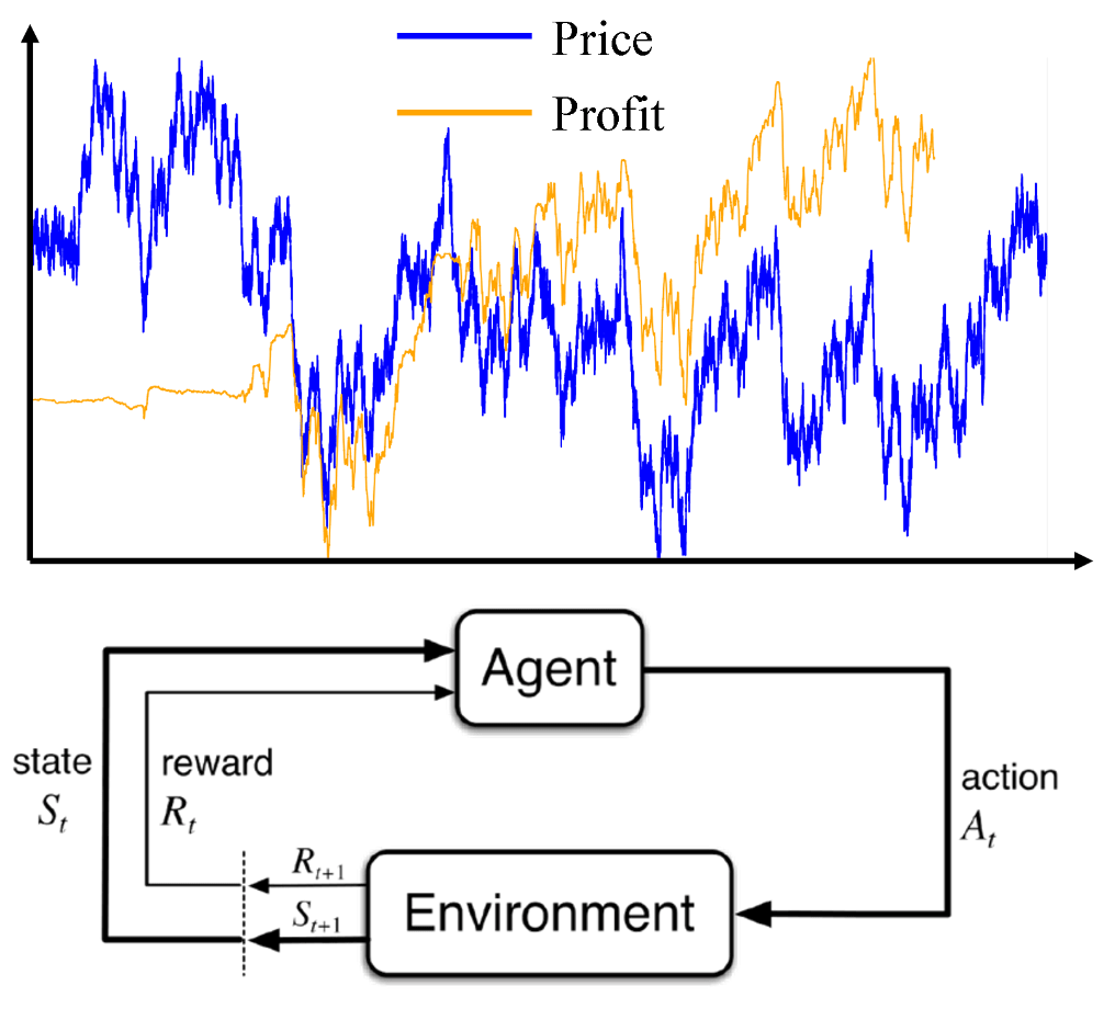
The model runs on a Windows 10 OS (i9-9900K CPU) with DDR4 2666MHz 16G RAM and NVIDIA GeForce RTX 2060 GPU. Tensorflow is used for constructing the artificial neural network (ANN), and a multilayer perceptron (MLP) is used. The code is modified from the Frozen-Lake example of reinforcement learning using Q-Networks. The model training process follows the Q-learning algorithm (off-policy TD control), which is illustrated in Fig. 1.
Figure 1. Algorithm for Q-learning and the agent-environment interaction in a Markov decision process (MDP) [1].
For each step, the agent first observes the current state, feeds the state values into the MLP and outputs an action that is estimated to attain the highest reward, performs that action on the environment, and fetches the true reward for correcting its parameters. The agent follows the epsilon-greedy policy (ε = 0.1) for striking a balance between exploration and exploitation.
State, Action and Reward
For the 1st generation, price values at certain time points and technical indicators are used for constructing the states. The technical indicators used are the exponential moving average (EMA) and Bollinger bands (N=20, k=2), and time frames of 1, 5 and 15min are used with the last 10 time points being recorded. A total number of 36 inputs are connected to the MLP.
There are three action values for the agent: buy, sell and do nothing. The action being taken by the agent is determined by the corresponding three outputs of the MLP, where sigmoid activation functions are used for mapping the outputs to a value range of 0 ~ 1, representing the probability of the agent taking that action.
For the reward function, the difference between the trade price (the price when a buy/sell action is taken) and the averaged future price is considered. If a buy action is taken, then the reward function is calculated by subtracting the averaged future price with the trade price; if a sell action is taken then the reward is calculated the other way around. For “do nothing” actions, the reward is 0. A spread is subtracted from the reward for buy/sell actions to obtain the final reward. This prevents the agent to perform actions that result in insignificant profit, which would likely lead to a loss for real trades (Fig. 2).
Figure 2. Reward calculation method for buy/sell actions.
Noisy Sine Function Test
For preliminary verification of effectiveness for the training model and methods, a noisy sine wave is generated with Brownian motion of offset and distortion in frequency. This means at a certain time point (min), the price is determined by the following equation:
where Pbias is an offset value with Brownian motion, Pamp is the price vibration amplitude, T is the period with fluctuating values, and Pnoise is the noise of the price with randomly generated values. (Note that the “price” mentioned here is defined as the exchange rate between two currencies)
Fig. 3 shows a randomly generated price vs time sequence within a range of 50,000 minutes with an initial values Pbias = 1.0, T = 120 min, Pamp = 0.005, and Pnoise amplitude = 0.001. Generally, the price seems to fluctuate randomly with no obvious highs or lows. However, if it is viewed close-up, waves with clear highs and lows can be observed (Fig. 4).
Figure 3. Price vs time of the noisy sine wave from 0 to 50,000 min.
Figure 4. Price vs time of the noisy sine wave from 20000 to 20600 min.
The whole time period is 1,000,000 min (approximately 700 days, or 2 years). Initially, a random time period is set for the environment. Every time the agent takes an action, there is a certain chance (= 1%) that the time will jump to another random point within the whole period. Otherwise, the time will move on to a random point which is around 1 ~ 2 day(s) in the future. This setting is expected to correspond to real conditions, where a profitable strategy can have stable earnings and can also adapt quickly to rapid changing environments.
Fig. 5 plots the cumulative profit for trading using the noisy sine wave signal for 50,000 steps. Although it took approximately 25,000 steps to make the model get “on track”, I recognize this result as an important start for implementing real data.
Figure 5. Cumulative profit from trading using a noisy sine wave signal.
Fundamental Analysis for Economic Events
Fundamental analysis is a tricky part in forex trading, since economic events not only correlate with each other, but also might have opposite effects on the price at different conditions. In this project, I extracted the events that are considered significant, and contain previous, forecast and actual values for analysis. Data from 14 countries of the past 10 years are downloaded and columns with incomplete values are abandoned, making a complete table of economic events.
Because different events have different impacts on forex, the price change after the occurrence of an event is monitored, and a correlation between each event and the seven major pairs (commodity pairs). Table 1 displays a portion of the correlation table for different economic events. The values are positive, which indicates the significance of an event on the currency pair. Here, a pair is denoted by the currency other than the USD (e.g. USD/JPY is denoted as JPY).
Table 1. Correlation table between 14 events and 5 currency pairs. Here, a pair is abbreviated as the currency other than the USD.
Country
Economic Event (Index)
AUD
CAD
EUR
GBP
JPY
AUD
Commodity Prices
0.00313
0.00268
0.00266
0.00339
0.00278
AUD
MI Inflation Expectations
0.00338
0.00168
0.00217
0.00200
0.00266
AUD
RBA Interest Rate Decision
0.00428
0.00262
0.00258
0.00298
0.00225
EUR
Manufacturing PMI
0.00331
0.00284
0.00263
0.00298
0.00278
EUR
Italian CPI
0.00315
0.00319
0.00295
0.00316
0.00255
EUR
Services PMI
0.00341
0.00290
0.00293
0.00295
0.00284
EUR
CPI
0.00304
0.00294
0.00262
0.00317
0.00241
EUR
German Unemployment Rate
0.00315
0.00315
0.00273
0.00313
0.00246
EUR
ECB President Trichet Speaks
0.00344
0.00248
0.00341
0.00302
0.00268
EUR
German Unemployment Change
0.00313
0.00313
0.00268
0.00307
0.00243
EUR
German Trade Balance
0.00306
0.00255
0.00300
0.00284
0.00268
EUR
German Factory Orders
0.00292
0.00265
0.00312
0.00280
0.00275
EUR
German Retail Sales
0.00304
0.00304
0.00353
0.00310
0.00275
EUR
French Trade Balance
0.00312
0.00312
0.00296
0.00301
0.00299
A total of 983 events are analyzed. However, due to the fact that a large portion of events have little influence on the price, only 125 events that have a relatively significant impact are selected as the inputs of the MLP.
Real Data Implementation Results
Per-minute exchange rate data of the seven currency pair is downloaded from histdata.com. A period from 2010 to 2019 is extracted, and blank values are filled by interpolation. This gives us a total of approximately 23 million records of price data (note that weekends have no forex data records), and is deemed sufficient for model training. The data is integrated into a table, and technical indices are calculated using ta, a technical analysis library for Python built on Pandas and Numpy.
Figure 6. EUR/USD exchange rate from 2010 to 2019.
Summing the inputs from technical analysis, fundamental analysis, and pure price data, a total of 1049 inputs are fed into the MLP. Within the hidden layers, ReLU activation is used, and a sigmoid activation function is used for the output layer. The output has a shape of 7×3, which represents the probability of the seven currency pairs and the three actions (buy, sell, do nothing).
Fig. 7 shows the accumulative profit from 2,000,000 steps in a single episode and its win rate (percentage of profitable trades within a moving average). An increasing spread value from 0.00001 to 0.00004 is applied, which the spread value starts from 0.00001 and increases by 0.00001 every 50,000 step. It can be seen that overall, the accumulative profit rises steadily. However, the win rate usually falls below the 50% line. How could a profitable trading strategy be possible? This is due to the fact that the average profit of a winning trade (=0.003736) is larger than the average loss of a losing trade (=0.003581). Thus, the overall result is a profitable trading strategy.
Figure 7. Accumulative profit and win rate from the training procedure of 2,000,000 steps.
Conclusion
In conclusion, a trading model for profitable forex trading is developed using reinforcement learning. The model can automatically adapt to dynamic environments to maximize its profits. Although for real conditions that have a larger spread, the model hasn’t achieved a stable and profitable result, the potential for optimizing is promising. In the future, I am planning to integrate this trading model with the automated forex trading system that I have made, and become a competitive player in this fascinating game of forex.
I have always wanted to automate the cumbersome experimental operation process. For biochemical experiments, often a whole day in web lab is spent in order just to acquire one single set of data. Having the hands-on experience of developing hardware and software integrated systems for several projects (e.g. Surface Plasmon Resonance Platform, Real-time Impedance Detection Systems), I initiated this project for constructing a microfluidic controlling platform that can automatically manipulate liquid-based solutions of little volume, and also assist real-time detection experiments.
Platform Structure
The platform is constructed by four sections: A Raspberry Pi, an actuator module that consists of an Arduino and two H-bridge circuits, a fluid controlling system made up of a syringe pump/syringe device, and the microfluidic platform (Fig. 1).
Figure 1. System architecture of the automated microfluidic controlling platform.
Here, the Raspberry Pi serves as the main processing unit, which an Apache web server is constructed on, and is used to communicate with a remote user by website. The front-end of the website is designed using HTML, Javascript and CSS, and the back-end is designed using PHP. Javascript and PHP communicate using jQuery, and the PHP code is written for controlling peripheral devices.
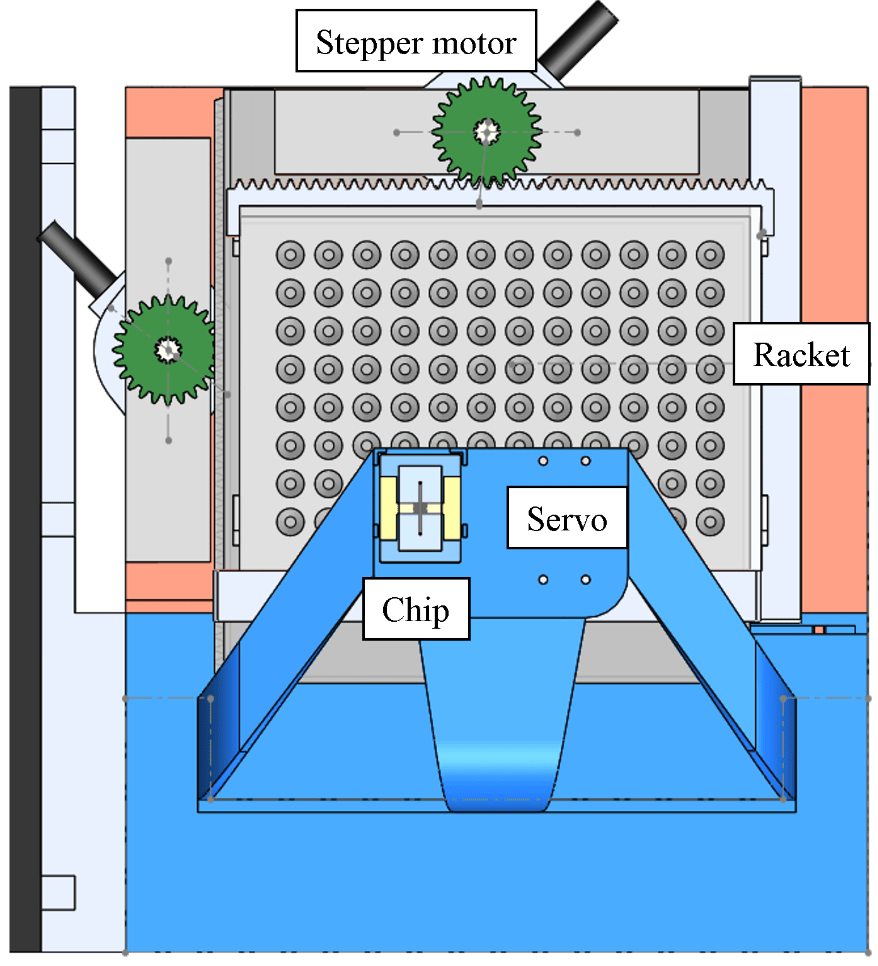
For x/y position control, the Raspberry Pi sends data through type-B USB to the Arduino, which afterwards commands the H-bridge circuits, then control the x/y stepper motors on the microfluidic platform for moving the position of the racket. The servo motor is used to control the high/low position of the tube it holds, where the high (low) position means the tube isn’t (is) inserted into the microtube (Fig. 2).
Figure 2. The microfluidic platform and surrounding modules.
For fluid control, the Raspberry Pi sends an infuse/withdraw signal to the syringe pump using another type-B USB, which subsequently pushes/pulls the syringe on it. A simple flow for moving liquid from microtube A to microtube B is:
1. Confirm that the tube (for fluid conveyance) position is high. If not, then move it up by servo motor. 2. Move to microtube A by stepper motor. 3. Change tube position to low by servo motor. 4. Withdraw liquid by syringe pump. 5. Change tube position to high by servo motor. 6. Move to microtube B by stepper motor. 7. Change tube position to low by servo motor. 8. Infuse liquid by syring pump.
Figure 3. Photograph of the automated microfluidic controlling platform.
The circuitry for this platform is relatively easy compared with other projects (e.g. Aroma Alarm Clock), and is consisted simply with wires and resistors. Except the motors and the racket with microtubes, all the other components of the for microfluidic platform are fabricated using 3D printing. 3D-printed gears are fixed with the stepper motors. Precise control of racket position (~ 0.2mm) is realized by combining the gears with a 3D-printed linear gear that fits on the racket and another linear gear of a subsidiary platform which the racket sits on. Below is a clip demonstrating how the 3D-printed components, the stepper motors, the racket with microtubes, and a microfluidic electrode chip are integrated together, along with x/y position control of the racket.
Software Development
The program structure written inside Raspberry Pi is quite similar to the program structure in another project “Real-time Impedance Detection Systems”. The difference for this project is that PHP is used to directly communicate with peripheral devices (Fig. 1).
Fig. 4 displays the website-based user interface for controlling this platform. The UI is divided in four sections: procedure window, buttons field, racket window, and status window. Briefly, the user can save/load settings from the connected Arduino, add/delete a control command, start/pause/stop the current procedure, download the control procedure to a text file, and append a command after another one.
Figure 4. Website user interface of the platform.
Fig. 5 shows the settings menu. Here, the user needs to find the device url for Arduino and the syringe pump beforehand and insert them. Several controlling preferences, such as motor operation delay time, steps for the stepper motor to move per cell (microtube), precise high/low position of the servo motor, current cell of the racket … etc. can be set.
Figure 5. Settings menu of the UI.
Fig. 6 shows the add command menu. The user can either move the stepper motor to a target cell (microtube), infuse/withdraw fluid at a self-defined rate and target volume, move servo high/low position, or perform a time delay.
Figure 6. The add command menu of the UI.
Concentration Gradient Generation
An automated concentration gradient generation process is written, and is carried out by the automated platform. Here is a clip for demonstration (speed = 10x):
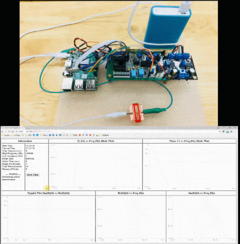
Real-time Impedimetric Detection
The tube doesn’t have to directly connect to a syringe. A detection chip can be inserted between for real-time detection of different solutions (similar to the method illustrated in Fig. 1 of another project Surface Plasmon Resonance Platform). A microfluidic interdigitated electrode chip using microfabrication technique is previously developed (which is a part of my research), and is used for detection of electrochemical impedimetric properties of the fluid. Here, potassium ferricyanide (K3Fe(CN)6) and potassium ferrocyanide (K4Fe(CN)6) are serial diluted using the platform, and real-time impedance detection is carried out using an electrochemical analyzer (CHI614b, CH Instruments) and the microfluidic chip.
Fig. 7 shows the detection result. It can be seen that the solution switching time is relatively fast and stable, and the detection time is consistent, which demonstrates the advantages of this automated platform.
Figure 7. Real-time impedimetric detection plot for different diluted concentrations of K3Fe(CN)6/K4Fe(CN)6.
Summary
In summary, a website-controlled automatic microfluidic controlling platform is designed and fabricated for real-time microfluidic sensing and other applications. Solution manipulation using this platform is stable, repeatable, and time-saving compared with manual operation.
This project is an integration of computer vision, mechatronics, wireless communication (Bluetooth), database management, mobile app design, sensors and actuators, and is a final project of a course called Design of Automated Systems. I teamed up with two classmates for accomplishing this challenging task of constructing a remote commandable car that can automatically detect and find balls with different colors, then be manually navigated towards a certain location. My contributions to this project are coding the ball-tracking algorithm using OpenCV, utilizing the microcontroller Arduino for movement control, and wiring electric components to the hardware circuit (yellow shaded area in Fig. 1).
System Architecture
Fig. 1 illustrates the system architecture for this project. Raspberry Pi is used as the main computer. Node.js is installed for communicating with the MariaDB database, receiving ordering signals from a remote Android app, and commanding the ball-tracking C++ program.
Figure 1. System architecture of the remote commandable self-driving toy car.
A standard procedure for command and action of the system is as follows.
Android user logins to Node.js server by verification of username and password through the database.
The user sends target ball color to the server.
The server sends command to “face_ball” program by bash.
“face_ball” detects colored ball position by ball recognition algorithm.
“face_ball” sends command to Arduino by serial USB.
Arduino controls two servo motors for the car to move towards the target ball.
After getting close enough, a fence is set to physically trap the ball.
Hardware Design
Fig. 2 shows a 3D drawing of the toy car. Components such as Arduino, Raspberry Pi (RPi) are fixed to the laser-cut acrylic board using plastic columns. Here, three servo motors are used. The first two controls the left/right wheel, and the third controls a trap that can lock the ball at the front of the car.
Figure 2. 3D illustration of the remote commandable toy car.
Figure 3. Preliminary version of the toy car.
Ball-Tracking Program
The main objective of the ball-tracking program is to navigate the toy car towards a target ball, and trap it with a fence connected to the toy car. The flowchart for image recognition of the ball is shown in Fig. 4.
Figure 4. Flowchart for the ball detection algorithm.
Using the above algorithm, rapid detection of the target ball can be realized. Here’s a demonstration of the program recognizing a ball being thrown in the air in real-time.
For movement control of the toy car, the Arduino will either turn left, turn right, or move straight according to the control algorithm shown in Fig. 5.
Figure 5. Flowchart for the ball-trapping algorithm.
Fig. 6 shows the commands available for controlling the toy car using Arduino.
Figure 6. Available commands for Arduino.
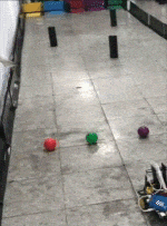
Here’s a clip for automated control of the toy car. A red ball is defined as the target and is trapped by the car using a fence.
Android App Design
The app is designed using MIT App Inventor, which implements a block-based programming method in which developers can create procedures by dragging predefined blocks together to for performing a certain function. Fig. 7 shows an image containing the complete code for the Android app. The user interface and flowchart for direct control of the toy car is shown in Fig. 8.
Figure 7. Complete block code for the Android app (click for magnified view).
Figure 8. App interface (left) and Arduino control flowchart (right).
Here’s a demonstration for the remote commandable toy car. The car automatically detects a green ball, moves near, and traps it. Then it is manually controlled to avoid obstacles and reach a yellow-colored area at the end.
As an old saying goes, “An hour in the morning is worth two in the evening”. What we encounter and conceive during this period is largely intertwined with our whole day. However, what is the most important thing that we encounter in the morning? It is about waking up. Nowadays, we wake up by the noisy, buzzing sound of an alarm. How would it be like if we could wake up by a scent, a fragrance, wiping away the unsatisfactory memories of the past? What can be changed to fulfill a better awakening?
An aroma alarm clock should fill in the answer. When I was a junior, I enrolled in a program called “NTU Creativity and Entrepreneurship Program” (NTUCEP). In this program, students with similar ideas form groups and learn about entrepreneurship by practice. After a couple days of brainstorming, our group came up with the concept about developing an alarm clock that can wake people up using scent packs. Apart from being awakened by a loud ringing sound of an alarm, fragrances (as we had proposed) have a milder, progressive effect for waking people up. We named our product “Sensio”, a Latin noun of the meaning “thought”.
Market Survey
In order to verify the market demand of this proposal, we devised a questionnaire for investigating the views and habits of people about waking up, which 1320 valid responses were collected. A score of 0 ~ 7 is used to quantify the “discomfort level” for waking up, in which a level of 0 ~ 3 is regarded as painless, and 4 ~ 7 as painful. Fig. 1 shows the discomfort level distribution of all the samples, and Fig. 2 shows the distributions by occupation. It can be seen that regardless of identity, the majority of people feel painful when waking up (students: 71%, office worker: 62%, other: 51%, overall: 68%). Moreover, we analyzed their habits of lying in bed after awakening. Fig. 3 shows the proportion and durations for lying in bed. Accordingly, over 44% of people lie in bed for over 15 minutes, and the average duration is 15.07 minutes. Theoretically, this means if a product could help lower one’s discomfort level of waking up, and reduce the duration of lying in bed after awakening, he could approximately increase 3.8 days/year of effective time. Not only having a favorable morning, but also enhancing his work efficiency.
Figure 1. Discomfort level distribution of waking up.
Figure 2. Number of people vs discomfort level by occupation.
Figure 3. Duration of lying in bed after awakening.
From the above analysis, we became confident about the large market demand for a better quality of getting up. For me, being the leading engineer role in our group of six meant turning ideas into reality. This had been a difficult period but a time of inspiration and excitement. I put into practice what I had learned within the past few years for developing a system, a hardware that can really be used as a product.
Sensio v0.1
I developed two preliminary versions of the hardware, with the 1st version using Arduino as the CPU (Sensio v0.1) (Fig. 4). In this version, an Arduino chip, a time clock module (DS1302), a shift register (74HC595N), relays, button switches, LED displays, a buzzer, a fan and a potentiometer are used for the alarm clock (Fig. 5). 10 different themes are written inside the system and a few simple features are integrated within (Fig. 6 details every mode of the alarm clock and the corresponding function of the buttons). This version serves as the proof-of-concept version for making an aroma alarm clock. Although being simple and somewhat rough, it demonstrated to my team and our professors a solid proof and feasibility of our objective.
Figure 6. Alarm modes and button function for Sensio v0.1.
During this period, we earned 40,000NTD in a fundraising event in our program, and won the Best Potential Award in the 14th NTU innovation competition. Fig. 7 shows the poster we had used in the competition. During that period, we had great enthusiasm and motivation, and dreamed that one day our product would become on-sale and we could establish a real listed company of our own. We entered the NTU garage, which is an incubator for startups that are closely linked to NTU.
Figure 7. Poster of product Sensio for the NTU innovation competition.
Sensio v0.2
The second version Sensio v0.2 was created during my second semester as a junior. This time, an IC chip (ATMEGA328P) is used as the CPU rather than Arduino in order to lower the cost of the system and decrease its volume. Moreover, a PCB layout for fixing electronic parts on a solid panel is used. Fig. 8 illustrates the structural model of Sensio v0.2, Fig. 9 shows a photograph of the integrated electric components and its corresponding PCB layout schematic, and Fig. 10 shows photographs of the laser-cut 3D outer case.
Figure 9. Electronic component-integrated PCB board of Sensio v0.2 and its corresponding layout schematic.
Figure 10. Outer case (blue) and scent pack holder (orange) of Sensio v0.2.
We were thrilled after these accomplishments, since never had a team of the same period achieved such a high level of completeness, especially when concerning the integrity of hardware and software. These remarkable things happen so quickly, so fleeting for us to catch up with. The truth is, we are still so far from success, since we were still students back then. Reality pulled us back, and we started asked ourselves: are we ready to give up some things and dedicate ourselves to entrepreneurship? Our dream product, the aroma alarm clock, had once seemed so close, yet had never seemed so far.
Although in the end, the functional aroma alarm clock wasn’t successfully made, what I’ve learned during this event is unprecedented compared with my past experience, not only techniques for hardware and software development, but also important philosophies for entrepreneurship. This project inspired me to a great extent, and enabled me for creating future hardware-related projects (e.g. Automated Microfluidic Controlling Platform, Real-time Impedance Detection Systems, Surface Plasmon Resonance Platform) in my own field of research.