Category: 1 Person
Real-time Impedance Detection System α
Linear Algebra Calculation using Integrated Circuits
Even the simplest thing we recognize may seem increasingly difficult in another point of view. Take a simple arithmetic operation for example, if one wants to calculate the function y = ax + b with given a and b, he simply multiplies any number x with a, then adds b, and gets the answer. What if no multiplication and addition can be used? How can the calculation even be possible?
Computers can actually finish the task by implementing three fundamental logic operations: AND, OR, and NOT. Most of them can do these operations within a nanosecond. In this project, I constructed a circuit for performing a simple linear algebra calculation (Fig. 1) using only basic logic and storage circuits (Fig. 2) that can be realized using standard cells.

Figure 1. Formula to be calculated. (x0, x1, x2 are all 6 bit 2’s complementary integers)

Figure 2. Basic logic and storage circuits. (Note that other circuits (e.g. NAND, XOR) are also used in this project)
Here, x0, x1 and x2 equal the three 6-bit integer inputs (2’s complementary), so there are a total of 18 Boolean input values. The output is stored in a 16-bit integer. Therefore, the goal for this project is to construct a circuit that connects all of the 18 inputs and the 16 outputs, and perform the calculation.
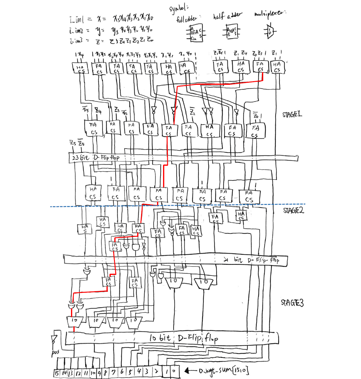
To make it harder, three stages of pipelines are carried out. This means that calculations are divided into three parts, and the most time-consuming part contains the critical path of the whole circuit. Fig. 3 shows an illustration of the designed circuit.

Figure 3. Logic circuit diagram for realizing the arithmetic operation (Fig. 1) of this project.
Verilog is used for simulating the results, and the circuit is written as a spice sub-circuit model. Because the D flip-flop is used, the critical time is defined as the clock cycle of the D flip-flop. Moreover, the number of transistors are defined for every basic logic circuit, so the total number of transistors can be calculated, and is named the “area” of the whole circuit.
Fig. 4 shows the simulation results of the circuit. It can be seen that only 1.3305 nanosecond is used for a half clock cycle of the circuit. This means that the circuit can continuously output calculation results every 2.661 nanosecond, which is really fast!

Figure 4. Simulation results using Verilog.
Having the experience of using absolutely no arithmetic operations for calculating a linear algebra problem really significantly broadened my insight towards digital IC design. This project inspired me to understand that even the most insignificant elements possess the potential to be combined and make up the world that we live in.
Guess the Number (iOS)
This is the first iOS game I had made using Xamarin, and is the second project of the guess the number series (after Guess the Number (Windows) and prior to Guess the Number AI). (The two-player game is also named Bulls and Cows.)
At the start of the game, a random 4-digit code is generated by the app and the player starts to guess that code. The player can restart the game anytime by pressing RESET, and a history of guesses and results are shown in a list at the bottom.
Here’s a demonstration of the app:
Considerations for app development are quite different from computer programs, such as the different screen sizes for different mobile platforms, and most of the time only a touch screen can be used. After finishing this project, I acquired some important fundamental concepts and know-hows for app design.
Guess the Number AI
After completing the first two projects of the Guess the Number series (Guess the Number (Windows) and Guess the Number (iOS)), I made an AI that can play this game at a high-human level.
It has been proven that at most 7 turns are needed to guess the answer, with a best average game length of 5.21 turns. For this game, all the possible combinations (e.g. “0123”, “7381” …) can be saved into a 1D array. After each guess, the possible combinations for the answer will be reduced. Therefore, the algorithm of the program is written for finding a number that will minimize the maximum possible combinations left. The time complexity for each turn is O(n3), and an average of 5 turns of guessing if needed for an arbitrarily chosen number.
For using the program, the user must first choose a 4-digit answer (e.g. “0123”), and input the two numbers [A] and [B] according to the game rules and the numbers guessed by the program. For instance, if the answer is “1357”, and the AI guesses “3127”, the user must input 1 2 ([A] = 1, [B] = 2).
Here’s a demonstration of the AI program guessing the answer “8192” in 5 guesses:
Nonogram AI
Nonograms (also known as Picross, Griddlers, Pic-a-Pix, and various other names) are picture logic puzzles, in which the cells in the grid must be colored or left blank according to the numbers on the side of the grid to display hidden pictures.

Figure 1. The initial and complete state of a 25×25 grid Nonogram.
(Source: https://www.nonograms.org/nonograms/i/32344 )
For a classical type of game, the numbers are a form of discrete tomography that measures how many unbroken lines of filled-in squares there are in any given row or column. For example, a clue of “1 2 3” would mean there are sets of one, two, and three filled squares, in that order, with at least one blank square between successive sets.
Solving Nonograms can be very time-consuming, and can be tremendously brain-twisting as the grid size increases, thus I created an AI program for automatically solving these puzzles.
The program utilizes the depth-first search algorithm that runs recursively from the top to bottom row. For the jth column of the ith row, the black or blank spaces must satisfy the tomographic rules formed by the numbers of the current row and column. This is a relatively simple approach for calculating the answer. However, because the algorithm does not solve the game using a more intuitive method for solving interrelated constraints, it will use a lot of time for big grids (over 40×40).
For the input format of this program, two numbers indicating the number of rows and columns are given first (n and m). Afterwards, there are n rows of data, with each row k starting with a number nk indicating how many numbers are given in that row, and followed by nk numbers representing the discrete tomography of black spaces of that very row; then there are m rows of data, and also starting with a number mk for the kth row, and followed by mk numbers representing the discrete tomography of black spaces for the kth column.
Here’s an example input for the Nonogram in Fig. 1:
25 25
1 8
2 7 3
1 16
2 11 4
2 13 2
2 14 2
1 18
2 8 4
2 6 4
2 5 5
3 4 2 2
3 4 3 1
3 3 2 1
2 3 2
2 3 2
3 2 1 4
3 2 1 4
3 2 1 4
3 3 1 4
2 5 4
1 11
1 10
1 5
1 5
1 6
1 1
1 2
1 2
1 4
1 11
1 13
1 15
2 9 3
2 8 3
3 7 5 2
3 7 3 4
3 6 2 3
3 8 3 2
2 13 2
2 10 2
3 5 5 3
4 4 1 4 6
4 1 2 2 8
3 3 1 10
4 3 1 4 4
4 2 1 2 3
3 2 1 2
2 2 1
2 2 1
1 1
A demonstration for using the AI program for solving a 39×50 Nonogram in about 22 seconds is shown below. The result displays an owl sitting on a branch (Fig. 2).

Figure 2. The complete state of a 39×50 Nonogram displaying an owl on a branch.
Othello AI
Othello (a variant of the traditional game Reversi) is a two-player strategy board game played on an 8×8 square field, where each player takes turns placing black or white pieces and capturing the other player’s pieces.

Figure 1. Othello board game.
The Othello AI program is the second board game AI that I have written in junior high school (the first is the Tic-Tac-Toe AI). Just like the programming strategy for the tic-tac-toe AI, I used the logic thinking experiences that I had learned while playing this game, and hard-coded some summarized strategies into this program.
Compared with the tic-tac-toe AI, which has a game-tree complexity of 9! = 362880, Othello is much more complex, yielding a stunning complexity of approximately 1058. This makes the game still mathematically unsolved up to this very day. Therefore, instead of calculating the definite winning strategy, this Othello AI rather tries to find relative advantageous points (e.g. the corners), and moves that will temporarily maximize the number of pieces which it occupies by the coded algorithm, making it a beginner ~ intermediate level AI.
Here is a demonstration of using the Othello AI program:
[Source code for the Othello AI program (Visual Basic 6.0 form file)]
Sudoku AI
Sudoku is a commonly known logic puzzle game, and had been one of my favorite puzzle games.
Having the experience for creating the simple Tic-Tac-Toe AI, I started to take on this challenge for creating an AI that can solve Sudoku.

Figure 1. The initial and complete board state of an expert-level Sudoku game.
I had written this AI program when I was in junior high school using Visual Basic 6.0. Having no prior knowledge for algorithms and data structures (which I learned in senior high school), I came up with a rough version of the backtracking algorithm myself, and implemented it on the AI. Here, the backtracking algorithm is a kind of depth-first search (DFS), and is guaranteed for finding a valid solution. Constraint programming is also integrated with the backtracking algorithm, since it is a very intuitive way for solving the puzzle.
Here is a clip demonstrating the Sudoku Solver program solving a hard-level Sudoku in around 5 seconds:
Here is another one that solved an expert-level Sudoku in around 44 seconds:
[Download program for the Sudoku Solver]
[Source code for the Sudoku Solver (Visual Basic 6.0 form file)]
Structural Biology Simulation
The usage of proteins is almost inevitable in most biochemical experiments. The ironic thing is, even if several billion or trillion proteins are present right in front of us, we never really get to see their true form due to their microscopic sizes. Thus, I enrolled in a class named structural biology, which I learned four programs: PyMOL, Swiss PDB Viewer, MolMol, and Chimera, for visualizing proteins, their physical properties, and several interaction mechanisms. This helped me understand important structural properties about the protein I had been studying.
Here I demonstrate some simulation methods implemented on the protein: signal transducer and activator of transcription 3 (STAT3). Three PDB files are used in this project: 3cwg, 1bg1, and 1bf5.
Analysis 1: Protein visualization using cartoon (top-left), dots (top-right), sticks (bottom-left) and spheres (bottom-right). Secondary structures such as the alpha helix and beta sheet are colored differently (PDB ID: 3cwg) (PyMOL).


Analysis 2: The volume of the protein (PDB ID: 1bg1) is calculated as 71.613nm3, and its surface area is calculated as 263.23nm2. The structure is transformed into a spherical molecular representation prior to calculation (Chimera).
Analysis 3: Total width and height of the protein (PDB ID: 3cwg) (Swiss PDB Viewer).

Analysis 4: Morphing between two different PDB files of the same protein (PDB ID: 3cwg and 1bg1) (Chimera). The blue structure is 3cwg, and the gray-white structure is 1bg1 in the lower figure.


Analysis 5: Electric charge on alpha helix (PDB ID: 3cwg) (PyMol).

Analysis 6: Mutation of Proline to Histidine at residue 255 (PDB ID: 3cwg) (Swiss PDB Viewer).


Analysis 7: Twisting of the ϕ and ψ angle (respectively left and right figure) at residue 255 (Proline) (PDB ID: 3cwg) (Swiss PDB Viewer).

ϕ angle 
ψ angle
Analysis 8: Ramachandran plots of the same protein with two different PDB files (PDB ID: 3cwg (left figure) and 1bg1 (right figure)) (MolMol).

3cwg 
1bg1
Analysis 9: Coulomb force on protein surface. The surface is colored from red (-10kcal/mol×e) to blue (10kcal/mol×e) gradient in order to indicate differences in Coulombic forces (PDB ID: 3cwg) (Chimera).
Analysis 10: The hydrogen bond between the two SH2 domains of the STAT3 dimer (PDB ID: 1bg1) (Chimera).

Analysis 11: Morphing between STAT3 (1bg1) and STAT1 (1bf5) (another similar protein of the STAT family) (Chimera). The blue structure is STAT1, and the white structure is STAT3 in the lower figure.


Fermentation Batch Reactor
For most of what we experience in everyday life, it is rare that one can directly link the obvious outcomes with their underlying theoretical grounds. Equations and plots seem such a long distance toward their practical applications. I regard this project as an important one which links observations of a simple experiment to the complex differential equations in reaction mechanics. This mini-project comes from a homework in reaction engineering, a course I had enrolled in during college. The experiment is simple that any person can carry out using easily accessible materials. The main objective is to construct a batch reactor that can exhibit fermentation with yeast, then quantify the reactions using what we have learned on class. (~age 21, 2017)
Two commercially available sugar-sweetened beverages, glucose solution, and water are used to explored how the sugar content in them affects the fermentation rate of rapid yeast. The anaerobic fermentation of yeast in anaerobic environment is:
C6H12O6 (monosaccharide) → 2C2H5OH (ethanol) + 2CO2 (carbon dioxide) + 2ATP
In this experiment, glass containers are filled with the solutions, then instant yeast is added the each container for production of carbon dioxide. A balloon is used for trapping the gases and is used as a volume sensor, where its dimensions are measured for calculating the volume of generated CO2. The molar concentration of CO2 is calculated using the ideal gas equation PV = nRT, and the ethanol production rate is calculated by relating with the proposed reaction and using finite different method.

Figure 1. Snapshots of balloon-sealed containers with added yeast at different times.

Figure 2. Volume of balloon (Vballoon) vs time (min).
Assume an inner air pressure of P = 1atm, a temperature of T = 310K (37°C). From the ideal gas equation, the relationship between the number of moles of CO2 and its volume is n = 3.931×10⁻⁵V, which according to the reaction, also equals the number of moles of ethanol. The molar concentration of ethanol is calculated by dividing the number of moles by its volume. And by using finite difference method of the first derivative, the rate of increase for molar concentration of ethanol (rC2H5OH) is calculated (Fig. 3).

Figure 3. Increase rate of molar concentration of ethanol (rC2H5OH) vs time (min).
It can be seen that in addition to pure water (Negative), the other three sugar-containing solutions have a maximum formation rate at the beginning (marked by the blue arrow). Wherein the ethanol production rate of glucose solution is eventually lower than 0(mM/min), it is presumed either this is caused by measurement errors or that carbon dioxide is dissolved back into the liquid, causing a decrease in volume, not a decrease in the amount of ethanol.
Here the production rate of ethanol in glucose solution started at a very high value (8.29mM/min), followed by fruit tea (4.17mM/min), and then raspberry juice (3.36mM/min). However, the sugar concentration of raspberry juice is higher than that of fruit tea. There are two factors that may be affected: the type of sugar and the pH value. Among them, the pH of fruit tea is between 5.0 and 6.0 and the pH of raspberry juice is between 2.3 and 2.52. However, the optimal living environment pH of yeast is 4.5 to 5.0, so it is speculated that the acidic environment of raspberry juice inhibits the activity of yeast and reduces rC2H5OH. In addition, only glucose exists in the glucose solution, but there is sucrose in both raspberry juice and fruit tea. Sucrose can be broken down by the yeast and producing ethanol twice as much as the same concentration of glucose. This explains why the final balloon volume (408.69cm3) of fruit tea is greater than the final balloon volume of the glucose solution (361.03cm3).
As being a simple hands-on experiment, this project successfully delivered the knowledge and allowed me to learn the fundamentals through practice, by which creating a connection between reality and theory.