Logic Circuit Control for Number Display

Most people believe, including me, that programming is a powerful technique, and a lot of things in everyday life are realized by programming. However, being taken away this skill, what can still be achieved?

In this project, a logic circuit with complex functionality is built using only simple IC chips and circuitry. A 7-segment LED displays numeral from 0 to 9 with adjustable frequency using a potentiometer, and the number can be reset anytime to 0 by pressing a reset button. For programmers utilizing a simple development board such as Arduino, this seems like a piece of cake. However, it requires a certain degree of knowledge for digital circuit and IC chip control in order to accomplish it without coding.

Here, two simple IC chips are used: a 4024 counter and a 4511 BCD to 7-segment converter. An oscillator circuit with square wave output and potentiometer-controllable frequency is constructed, and the signal is fed into the 4024 counter, which outputs bitwise data to the 4511 converter, and eventually sends to the 7-segment display. A latch circuit and button is connected to the reset input of the 4024 counter for adding the reset function.

I was fascinated by the wide applicability of digital circuits, which can achieve low-cost and stable hardware features such as this project.

Here’s a video demonstration of this project (note that the Arduino on the left is just for power supply):

Structural Biology Simulation

The usage of proteins is almost inevitable in most biochemical experiments. The ironic thing is, even if several billion or trillion proteins are present right in front of us, we never really get to see their true form due to their microscopic sizes. Thus, I enrolled in a class named structural biology, which I learned four programs: PyMOL, Swiss PDB Viewer, MolMol, and Chimera, for visualizing proteins, their physical properties, and several interaction mechanisms. This helped me understand important structural properties about the protein I had been studying.

Here I demonstrate some simulation methods implemented on the protein: signal transducer and activator of transcription 3 (STAT3). Three PDB files are used in this project: 3cwg, 1bg1, and 1bf5.

Analysis 1: Protein visualization using cartoon (top-left), dots (top-right), sticks (bottom-left) and spheres (bottom-right). Secondary structures such as the alpha helix and beta sheet are colored differently (PDB ID: 3cwg) (PyMOL).

Analysis 2: The volume of the protein (PDB ID: 1bg1) is calculated as 71.613nm3, and its surface area is calculated as 263.23nm2. The structure is transformed into a spherical molecular representation prior to calculation (Chimera).

Analysis 3: Total width and height of the protein (PDB ID: 3cwg) (Swiss PDB Viewer).

Analysis 4: Morphing between two different PDB files of the same protein (PDB ID: 3cwg and 1bg1) (Chimera). The blue structure is 3cwg, and the gray-white structure is 1bg1 in the lower figure.

Analysis 5: Electric charge on alpha helix (PDB ID: 3cwg) (PyMol).

Analysis 6: Mutation of Proline to Histidine at residue 255 (PDB ID: 3cwg) (Swiss PDB Viewer).

Analysis 7: Twisting of the ϕ and ψ angle (respectively left and right figure) at residue 255 (Proline) (PDB ID: 3cwg) (Swiss PDB Viewer).

Analysis 8: Ramachandran plots of the same protein with two different PDB files (PDB ID: 3cwg (left figure) and 1bg1 (right figure)) (MolMol).

Analysis 9: Coulomb force on protein surface. The surface is colored from red (-10kcal/mol×e) to blue (10kcal/mol×e) gradient in order to indicate differences in Coulombic forces (PDB ID: 3cwg) (Chimera).

Analysis 10: The hydrogen bond between the two SH2 domains of the STAT3 dimer (PDB ID: 1bg1) (Chimera).

Analysis 11: Morphing between STAT3 (1bg1) and STAT1 (1bf5) (another similar protein of the STAT family) (Chimera). The blue structure is STAT1, and the white structure is STAT3 in the lower figure.

Fermentation Batch Reactor

For most of what we experience in everyday life, it is rare that one can directly link the obvious outcomes with their underlying theoretical grounds. Equations and plots seem such a long distance toward their practical applications. I regard this project as an important one which links observations of a simple experiment to the complex differential equations in reaction mechanics. This mini-project comes from a homework in reaction engineering, a course I had enrolled in during college. The experiment is simple that any person can carry out using easily accessible materials. The main objective is to construct a batch reactor that can exhibit fermentation with yeast, then quantify the reactions using what we have learned on class. (~age 21, 2017)

Two commercially available sugar-sweetened beverages, glucose solution, and water are used to explored how the sugar content in them affects the fermentation rate of rapid yeast. The anaerobic fermentation of yeast in anaerobic environment is:

C6H12O6 (monosaccharide) → 2C2H5OH (ethanol) + 2CO2 (carbon dioxide) + 2ATP

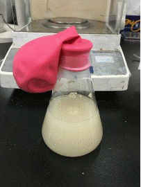
In this experiment, glass containers are filled with the solutions, then instant yeast is added the each container for production of carbon dioxide. A balloon is used for trapping the gases and is used as a volume sensor, where its dimensions are measured for calculating the volume of generated CO2. The molar concentration of CO2 is calculated using the ideal gas equation PV = nRT, and the ethanol production rate is calculated by relating with the proposed reaction and using finite different method.

Figure 1. Snapshots of balloon-sealed containers with added yeast at different times.

Figure 2. Volume of balloon (Vballoon) vs time (min).

Assume an inner air pressure of P = 1atm, a temperature of T = 310K (37°C). From the ideal gas equation, the relationship between the number of moles of CO2 and its volume is n = 3.931×10⁻⁵V, which according to the reaction, also equals the number of moles of ethanol. The molar concentration of ethanol is calculated by dividing the number of moles by its volume. And by using finite difference method of the first derivative, the rate of increase for molar concentration of ethanol (rC2H5OH) is calculated (Fig. 3).

Figure 3. Increase rate of molar concentration of ethanol (rC2H5OH) vs time (min).

It can be seen that in addition to pure water (Negative), the other three sugar-containing solutions have a maximum formation rate at the beginning (marked by the blue arrow). Wherein the ethanol production rate of glucose solution is eventually lower than 0(mM/min), it is presumed either this is caused by measurement errors or that carbon dioxide is dissolved back into the liquid, causing a decrease in volume, not a decrease in the amount of ethanol.

Here the production rate of ethanol in glucose solution started at a very high value (8.29mM/min), followed by fruit tea (4.17mM/min), and then raspberry juice (3.36mM/min). However, the sugar concentration of raspberry juice is higher than that of fruit tea. There are two factors that may be affected: the type of sugar and the pH value. Among them, the pH of fruit tea is between 5.0 and 6.0 and the pH of raspberry juice is between 2.3 and 2.52. However, the optimal living environment pH of yeast is 4.5 to 5.0, so it is speculated that the acidic environment of raspberry juice inhibits the activity of yeast and reduces rC2H5OH. In addition, only glucose exists in the glucose solution, but there is sucrose in both raspberry juice and fruit tea. Sucrose can be broken down by the yeast and producing ethanol twice as much as the same concentration of glucose. This explains why the final balloon volume (408.69cm3) of fruit tea is greater than the final balloon volume of the glucose solution (361.03cm3).

As being a simple hands-on experiment, this project successfully delivered the knowledge and allowed me to learn the fundamentals through practice, by which creating a connection between reality and theory.

Gomoku AI

Although entering a department different from Computer Science (CS), I still had a majority of acquainted people in NTU-CS. One day, a friend of mine who was studying in CS challenged me of making an AI of some board game. The two of us would make AIs of that game and try to win the other one using the AI. Thinking it might be some challenging but interesting subject, I started to make this Gomoku AI.

Figure 1. Game playing demonstration of the Gomoku AI program.

Being a board game with so many possible states (more than the Othello AI I had made when I was in junior high school, which only has a 8×8 grid) , it is considered overly time wasting for the AI to traverse all the possible combinations, even just within 10 moves! Game tree graphs, graph traversal algorithms (e.g. DFS, BFS) and optimal searching algorithms (e.g. Alpha–beta pruning, A*) are usually implemented for decreasing computational time and achieving the best strategy. In this project, I only used the depth-first search (DFS) algorithm, along with some hard coded optimization decisions to create this program. Although being able to place a few initial pieces successfully, the program suffers from a large amount of computational time being spent. Most of the time after a few moves, the program will just run for a few hours (or days) before taking the next move, which is obviously very a serious problem for the AI.

Nevertheless, the environment and rules of the Gomoku game engine was successfully constructed, which allowed two players to play against each other. Nowadays, these board game AI are usually designed using deep neural networks, such as AlphaGomoku, an Alpha-Go-based Gomoku AI. Constructing these AIs would be a possible future work for optimizing this game agent.

NTU Library 3D Drawing

This is a model of the library of National Taiwan University (NTU) and was created using Solidworks. This project was originally a homework from the course “Engineering Drawing” of our department. Being fascinated by the features and functions provided by the 3D CAD drawing software, I took “the hard way” by choosing this architecture as the target for this homework.

Figure 1. Solidworks Components of NTU library.

Partial images were downloaded and pasted for being the surface material of individual components of the library. I searched for some 3D images of the library and managed to duplicate the outline and structures onto the parts (Fig. 1). Taking a large amount of effort constructing and assembling the pieces, I gained a lot of experience finishing this project. After completing this project, I learned some important concepts of 3D drawing which provided me to design other structures for 3D printing in further projects.

Figure 2. Diagonal view of the assembled NTU library.